


Consensus earnings estimates are widely presented as authoritative reference points. They are often interpreted as the market's collective expectation and used as benchmarks for evaluating reported results. The danger lies in the assumption that a single aggregated number reflects genuine agreement among analysts. In reality, consensus can conceal meaningful disagreement that materially alters how risk should be interpreted.
Consensus is not a singular viewpoint. It represents the aggregation of multiple independent forecasts produced by analysts operating with different models, assumptions, and information sets. The published figure is typically derived from an averaging process.
Aggregation creates clarity, but it also compresses dispersion. Two companies may display identical consensus EPS figures while exhibiting entirely different degrees of disagreement beneath the surface. Without examining the distribution of forecasts, the headline number does not distinguish between alignment and structural uncertainty.
This article examines consensus as a statistical construct rather than an informational signal. Using analyst estimate distribution data from Financial Modeling Prep (FMP), we analyze how dispersion across forecasts can provide deeper insight into uncertainty than the consensus mean alone.
How Consensus Is Constructed
Analyst consensus begins with individual earnings forecasts.
A broader overview of earnings analysis and how analyst projections fit into financial evaluation is available in FMP's guide to earnings and financial analysis fundamentals.
Equity research analysts publish projections for metrics such as earnings per share (EPS) and revenue for upcoming reporting periods. Each forecast reflects a distinct analytical framework, including assumptions about revenue growth, margins, cost structures, and macroeconomic conditions.
Data providers collect these individual estimates and aggregate them into summary statistics. The most commonly reported figure is the mean or median estimate for a given period. Alongside the consensus value, providers often publish the highest estimate, lowest estimate, and the number of contributing analysts.
The aggregation process produces a single reference number. This number is frequently treated as the expected outcome for the company. However, the consensus does not eliminate disagreement. It simply averages it.
Two structurally different situations can produce an identical consensus figure: broad agreement among analysts, or substantial disagreement that averages to the same mean.
For example, three analysts each projecting EPS of $2.00 generate a consensus of $2.00 with minimal dispersion. In contrast, one analyst projecting $1.00 and another projecting $3.00 also produce a consensus of $2.00. The headline number is identical in both cases, yet the second scenario reflects materially higher disagreement and therefore greater uncertainty around the expected outcome.
Without examining the distribution of estimates, the consensus value alone does not distinguish between alignment and divergence. The distribution carries information about uncertainty that the aggregated mean does not display.
Understanding this structure is essential before interpreting consensus as a signal. The mean summarizes forecasts. The dispersion describes them.
FMP API Endpoints Used
The analysis in this article relies on analyst estimate distribution data available through Financial Modeling Prep (FMP). The following endpoints are used in the workflow:
Financial Estimates API:This API provides forward-looking analyst projections, including:
- Consensus EPS and revenue estimates
- High and low estimate ranges
- Number of contributing analysts
- Period-specific estimate data
For additional context on interpreting forward-looking financial data, refer to FMP's educational resources on forecasting and financial projections.
These fields allow examination of both the aggregated consensus value and the distribution behind it.
The workflow below extracts the consensus estimate along with its high-low range and analyst count in order to evaluate dispersion directly.
How to Get Your API Key
To access Financial Modeling Prep's APIs, you need a valid API key.
Create an account using the official registration page.
After registration, your API key will be available in your dashboard. Replace "YOUR_API_KEY" in the code examples below with your personal key to authenticate requests.
Pulling Estimate Distribution Data (Python Workflow)
The objective is to examine the structure behind the consensus number. Specifically, we extract:
- Consensus EPS
- High estimate
- Low estimate
- Number of analysts
This allows direct observation of dispersion instead of relying solely on the aggregated mean.
Step 1: Fetch Analyst Estimate Data
|
import requests import pandas as pd API_KEY = "YOUR_API_KEY" symbol = "NVDA" url = ( f"https://financialmodelingprep.com/stable/analyst-estimates" f"?symbol={symbol}&limit=20&apikey={API_KEY}" ) response = requests.get(url) if response.status_code != 200: raise Exception(f"API request failed: {response.status_code} - {response.text}") data = response.json() df = pd.DataFrame(data) df.head() |

This retrieves forward-looking analyst EPS projections for the selected company.
Step 2: Select Relevant Fields
|
columns_needed = [ "symbol", "date", "estimatedEpsAvg", "estimatedEpsHigh", "estimatedEpsLow", "numberAnalystsEstimatedEps" ] estimates = df[columns_needed].copy() estimates.head() |
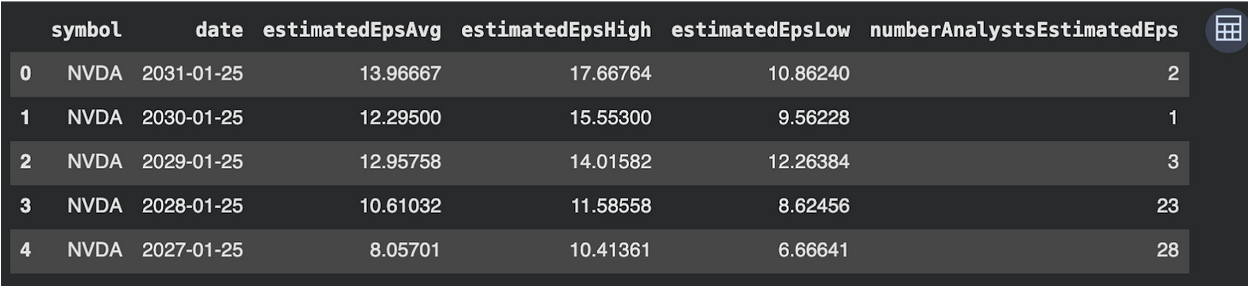
This subset retains the consensus EPS and its distribution bounds, along with the number of analysts contributing to the EPS estimate.
Step 3: Compute Dispersion Measures
|
# Absolute dispersion in EPS forecasts estimates["spread"] = estimates["estimatedEpsHigh"] - estimates["estimatedEpsLow"] # Dispersion scaled by consensus EPS (handles varying EPS levels across periods) estimates["relative_spread"] = estimates["spread"] / estimates["estimatedEpsAvg"] # Optional: keep output clean and consistent for interpretation estimates = estimates.sort_values("date", ascending=False) estimates.head() |

The relative_spread column expresses the forecast range as a proportion of the consensus EPS. Interpreting its magnitude requires contextual framing.
As a general heuristic, a relative spread below 0.10-0.15 often reflects relatively tight analyst alignment. Values between 0.20-0.30 indicate moderate disagreement. Levels approaching or exceeding 0.40 suggest materially elevated dispersion, meaning analysts differ widely in their forward expectations.
In the NVDA dataset above, relative spread reaches approximately 0.46-0.49 in later periods (2030-2031). This indicates that the high-low EPS range spans nearly half of the consensus average — a structurally wide distribution. In contrast, 2029 shows a relative spread near 0.13, reflecting comparatively tighter clustering of forecasts.
Importantly, the highest dispersion periods also coincide with lower analyst counts (1-2 contributors). Limited coverage can amplify proportional spread, increasing structural uncertainty in the consensus figure.
Relative spread therefore functions as a scale-adjusted uncertainty indicator. The consensus average alone does not convey this variation.
Step 4: Examine Dispersion Trends Over Time
Dispersion at a single point in time provides structural insight. Examining how dispersion evolves across reporting periods reveals whether disagreement among analysts is expanding or compressing.
|
# Ensure date is properly formatted estimates["date"] = pd.to_datetime(estimates["date"]) # Sort chronologically estimates = estimates.sort_values("date") # Measure period-over-period change in dispersion estimates["spread_change"] = estimates["spread"].diff() estimates["relative_spread_change"] = estimates["relative_spread"].diff() # Display most recent observations estimates.tail() |

The recent snapshot of estimate data shows meaningful fluctuation in dispersion across reporting periods. In later forecast horizons, relative spread expands materially after a period of compression. For example, relative dispersion declines to approximately 0.13 in one mid-horizon period before widening again toward roughly 0.48 in subsequent forward estimates.
This shift indicates that analyst disagreement does not move monotonically with the consensus average. Periods of tighter clustering can be followed by renewed divergence in forward projections.
The most distant forecast periods in the current dataset exhibit both elevated relative dispersion and reduced analyst participation. With only one or two contributing analysts, the proportional high-low range expands significantly. This combination reflects structural uncertainty embedded in longer-dated estimates.
These observations reflect the dataset at the time of analysis. As new estimates are published and analyst coverage evolves, dispersion levels may shift accordingly.
Step 5: Compare EPS and Revenue Dispersion
Earnings disagreement does not always originate from revenue assumptions. In some periods, revenue expectations cluster tightly while EPS estimates diverge due to margin or cost assumptions.
The following code evaluates dispersion for revenue alongside EPS.
|
revenue_cols = [ "date", "estimatedRevenueAvg", "estimatedRevenueHigh", "estimatedRevenueLow" ] revenue_estimates = df[revenue_cols].copy() # Compute revenue spread revenue_estimates["revenue_spread"] = ( revenue_estimates["estimatedRevenueHigh"] - revenue_estimates["estimatedRevenueLow"] ) # Convert date for alignment revenue_estimates["date"] = pd.to_datetime(revenue_estimates["date"]) # Merge with EPS dispersion combined = pd.merge( estimates, revenue_estimates[["date", "revenue_spread"]], on="date", how="left" ) combined.tail() |

The combined output reveals that dispersion in EPS forecasts does not always move in tandem with revenue dispersion.
For example, in one forward period, EPS relative_spread rises to approximately 0.48, meaning the high-low earnings range spans nearly half of the consensus EPS. During that same period, revenue_spread remains within a narrower directional range relative to adjacent periods and does not exhibit a proportionally similar expansion.
Earlier in the dataset, when EPS relative_spread compresses toward roughly 0.13, revenue dispersion does not decline to the same proportional extent. This asymmetry suggests that disagreement among analysts is concentrated more heavily in profitability assumptions than in top-line revenue expectations.
In practical terms, analysts appear relatively aligned on revenue trajectory while diverging on margin structure, cost assumptions, or operating leverage effects that ultimately drive EPS outcomes.
The dispersion differential therefore isolates the source of uncertainty: not whether revenue will grow, but how efficiently that revenue converts into earnings.
Step 6: Identify the Most Uncertain Reporting Periods
Ranking reporting periods by relative dispersion highlights where analyst disagreement is structurally elevated.
|
# Rank by highest proportional dispersion most_uncertain_periods = ( estimates .sort_values("relative_spread", ascending=False) .head(5) ) most_uncertain_periods[[ "date", "estimatedEpsAvg", "spread", "relative_spread", "numberAnalystsEstimatedEps" ]] |
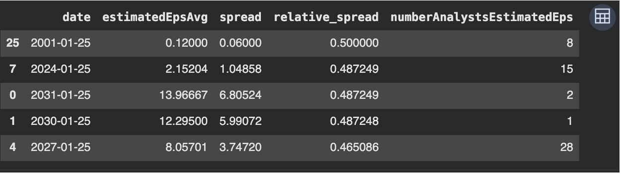
The ranking highlights reporting periods with the highest proportional dispersion in EPS forecasts. Several periods exhibit relative spreads near 0.48-0.50, indicating that the high-low estimate range spans nearly half of the consensus EPS.
Structural uncertainty increases when elevated dispersion coincides with low analyst participation. In periods where only one or two analysts contribute, the consensus and its high-low range become highly sensitive to individual forecasts. A single optimistic or conservative estimate can materially widen the range, amplifying proportional dispersion.
In contrast, when analyst coverage is broader — such as periods with 20+ contributors — the high-low range reflects a more statistically distributed set of independent views. Outlier influence is diluted across a larger sample, and dispersion more accurately reflects collective disagreement rather than individual forecast variance.
For example, in the dataset above, certain forward periods with only one or two contributing analysts display relative spreads near 0.49. While dispersion appears elevated, the small sample size increases sensitivity to individual assumptions. This makes the consensus structurally less stable than a similarly wide spread supported by broad analyst coverage.
Dispersion therefore interacts with analyst count. Wide ranges combined with limited participation signal heightened structural fragility in the consensus figure.
When Consensus Appears Stable but Dispersion Persists
The DataFrame above contains both the consensus estimate (estimatedEpsAvg) and the dispersion measures (spread and relative_spread).
Examining recent periods shows that estimatedEpsAvg may change only marginally across reporting dates. The headline consensus appears stable. However, the relative_spread column can remain elevated at the same time. This indicates that analysts continue to publish forecasts that differ materially from one another, even though the aggregated mean does not reflect that variation.
In practical terms, a stable consensus combined with high dispersion increases the probability of earnings surprises. If analyst forecasts are widely dispersed, the reported result is more likely to fall meaningfully above or below a large portion of estimates — even if it aligns closely with the mean. The consensus may appear steady, but disagreement beneath the surface implies uncertainty about the true earnings outcome.
The numberAnalystsEstimatedEps field adds further structure. A stable average combined with persistent dispersion suggests unresolved analytical disagreement rather than convergence. In such environments, earnings releases can trigger outsized reactions because market participants may anchor to the consensus mean while underestimating the breadth of forecast divergence.
The consensus figure summarizes forecasts. The distribution reveals their stability.
Why Dispersion Carries More Information Than the Mean
The DataFrame illustrates that similar values in estimatedEpsAvg can coexist with materially different values in spread and relative_spread. The consensus value alone does not convey this structural variation.
A narrow spread corresponds to clustering of forecasts around the average. A wide spread reflects dispersion of views across a broader interval between estimatedEpsHigh and estimatedEpsLow. The relative_spread metric scales that range against the level of the consensus EPS, allowing disagreement to be interpreted proportionally rather than in absolute dollar terms.
When estimatedEpsAvg remains stable but relative_spread expands, the consensus masks widening uncertainty. When numberAnalystsEstimatedEps declines at the same time, the structural stability of the consensus weakens further.
In the dataset above, the informational content does not reside in estimatedEpsAvg alone. It emerges from the interaction between the consensus value, its high-low range, proportional dispersion, and analyst participation. The mean provides a benchmark. The distribution fields reveal the confidence around that benchmark.
When Consensus Still Has Value
Consensus estimates retain practical utility when interpreted appropriately. The aggregated figure provides a standardized benchmark against which reported earnings are evaluated. It enables consistent comparison across companies and reporting periods.
The consensus value also serves as a reference point for tracking directional revisions over time. Sequential changes in estimatedEpsAvg reflect shifts in aggregate expectations, particularly when observed alongside historical estimate snapshots.
In comparative analysis, consensus facilitates alignment across peer groups. A single reference number allows analysts and researchers to position companies relative to prevailing expectations within a sector.
Its limitation lies not in its construction, but in its interpretation. Consensus functions effectively as a benchmark. It becomes incomplete when treated as a comprehensive representation of analyst agreement.
Evaluated together with dispersion measures and analyst participation, the consensus estimate forms part of a broader interpretive framework rather than a standalone signal.
Access to structured analyst estimate data, including high-low ranges and analyst participation metrics, is available through FMP's developer plans detailed on the FMP pricing page.
When Dispersion Can Mislead
Dispersion provides structural insight, but it is not universally definitive. Certain conditions can distort the interpretive value of spread and relative_spread.
Thin Coverage Periods
When numberAnalystsEstimatedEps is low, dispersion can be amplified by individual outliers. With only one or two contributing analysts, the high-low range may expand materially even if disagreement is not broadly distributed. In such cases, wide dispersion reflects sample sensitivity rather than collective uncertainty.
Highly Seasonal Earnings Cycles
Companies with pronounced seasonality may exhibit elevated forecast dispersion during off-cycle quarters. Analysts may diverge in short-term timing assumptions while maintaining similar full-year expectations. Temporary widening of relative_spread may therefore reflect timing variability rather than structural disagreement.
Structural Long-Term Growth Names
High-growth companies often experience naturally wider dispersion in forward periods. As forecast horizons extend, assumptions about revenue scaling, margin evolution, and capital intensity diverge. In such contexts, elevated relative_spread may reflect scenario modeling breadth rather than instability in near-term earnings expectations.
Dispersion should therefore be interpreted alongside analyst count, forecast horizon, and business model characteristics. The distribution adds perspective, but context determines whether wide ranges reflect structural risk or normal forecasting dynamics.
Conclusion
Consensus estimates are frequently interpreted as authoritative expectations. Their singular form creates an impression of clarity and agreement. In practice, consensus represents the aggregation of multiple independent forecasts.
Aggregation simplifies interpretation, but it also compresses variation. The average alone does not describe the degree of alignment or disagreement among contributing analysts. The distribution of estimates provides that context.
Treating consensus as a definitive signal overlooks the structural information embedded in the range of forecasts. A disciplined interpretation considers both the benchmark value and the variation beneath it.
Consensus remains useful as a reference point. The underlying distribution provides the perspective necessary to evaluate how stable that reference truly is.