Every algorithmic model depends on one thing: timely data.

Real-time market data refers to continuously updating prices, volumes, and indicators delivered directly from exchanges through APIs — essential for building responsive trading and analytics systems.

In modern systems, real-time market data flows straight from the feed into feature engineering, signal generation, and order routing. If the feed lags, momentum flips can be missed, spreads can close, and stops can slip.

With Financial Modeling Prep (FMP) you can stream stock market data feeds (quotes, intraday OHLCV, technical indicators) fast enough to power stock market data analysis, trading dashboards, and live strategies.

The diagram below shows how data flows through a modern trading workflow — from market feeds to execution and risk monitoring.

Figure 1 — Trading Workflow (ASCII)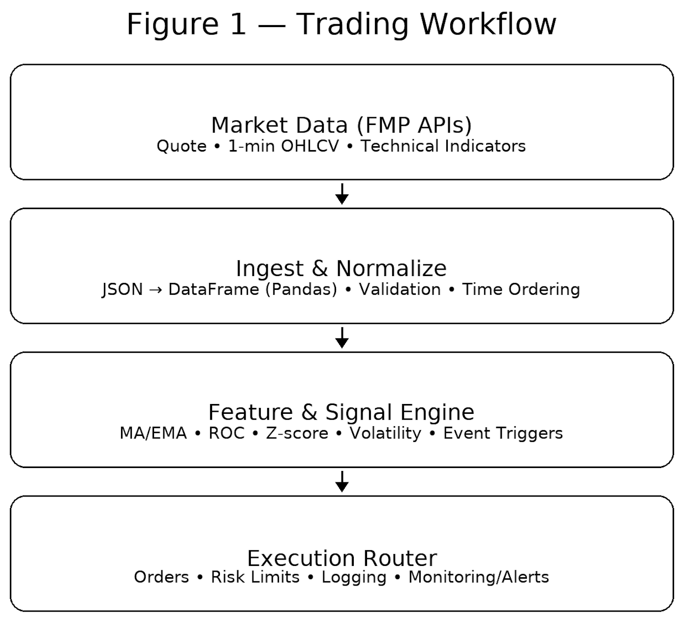

Let's break down how quants and traders transform live data into strategy.

How Traders Apply Real-Time Market Data

Real-time feeds enable short-horizon tactics where seconds (or less) matter. Below is a compact map of common strategies and their data needs.

Table 1 — Common Trading Strategies Using Real-Time Data

Strategy	Core Metric	Data Frequency	Goal
Momentum	Price change velocity (ROC/slope)	1s-1m	Capture continuation
Mean Reversion	Deviation from moving average	1m-5m	Profit from reversals
Arbitrage	Cross-market price gaps	<1s	Exploit mispricing

Momentum

Track short-term acceleration. With 1-minute AAPL data, compute ROC or a fast EMA slope; when slope and volume confirm, enter in the direction of strength and trail a dynamic stop.

Mean Reversion

Compare price to an intraday MA/VWAP. If AAPL travels >2σ above a 20-period 1-minute average, fade the move with tight risk and exit into the reversion.

Arbitrage

Monitor the same asset across venues or related pairs; execute when a micro-spread opens. This demands sub-second quotes and low-latency execution.

FMP Real-Time APIs You'll Use

Below are the endpoints we'll call and how they fit into trading data API workflows. These examples show how each API fits into a live trading workflow

1) Real-Time Stock Quote (snapshot)

Endpoint:

https://financialmodelingprep.com/stable/quote?symbol=AAPL&apikey=api_key

What it returns:

[ { "symbol": "AAPL", "name": "Apple Inc.", "price": 247.08, "changePercentage": -0.23419, "change": -0.58, "volume": 23258596, "dayLow": 244.7, "dayHigh": 248.82, "yearHigh": 260.1, "yearLow": 169.21, "marketCap": 3666763561200, "priceAvg50": 237.9244, "priceAvg200": 222.2168, "exchange": "NASDAQ", "open": 246.615, "previousClose": 247.66, "timestamp": 1760471369 } ]

How traders use it:

• Dashboard tiles (price, % change, volume).
• Sanity-check latency by comparing timestamp to local time.
• Regime filters (e.g., price vs. priceAvg50/200).

2) 1-Minute Intraday Chart (OHLCV stream)

Endpoint:

https://financialmodelingprep.com/stable/historical-chart/1min?symbol=AAPL&apikey=api_key

What it returns (sample from your spec):

[ { "date": "2025-10-14 15:48:00", "open": 247.05, "low": 246.93, "high": 247.1443, "close": 247.03, "volume": 51807 }, { "date": "2025-10-14 15:47:00", "open": 247.318, "low": 246.955, "high": 247.318, "close": 247.08, "volume": 66809 }, { "date": "2025-10-14 15:46:00", "open": 247.06, "low": 247.06, "high": 247.41, "close": 247.34, "volume": 113060 }, { "date": "2025-10-14 15:45:00", "open": 247.08, "low": 246.97, "high": 247.18, "close": 247.0447,"volume": 98632 } ... ]

How traders use it:

• Compute intraday features (EMAs, ROC, z-scores, ATR).
• Trigger tactics (breakouts, fades) on fresh bars.
• Build stock market data dashboards that refresh each minute.

3) EMA Technical Indicator

Endpoint:

https://financialmodelingprep.com/stable/technical-indicators/ema?symbol=AAPL&periodLength=10&timeframe=1day&apikey=api_key

What it returns (sample from your spec):

[ { "date": "2025-10-14 00:00:00", "open": 246.615, "high": 248.82, "low": 244.7, "close": 248.3398, "volume": 22398193, "ema": 251.49117773891516 }, { "date": "2025-10-13 00:00:00", "open": 249.38, "high": 249.69, "low": 245.56, "close": 247.66, "volume": 38142942, "ema": 252.19148390311852 }, { "date": "2025-10-10 00:00:00", "open": 254.94, "high": 256.38, "low": 244, "close": 245.27, "volume": 61999100, "ema": 253.19848032603377 } ... ]

How traders use it:

• Blend intraday signals with daily trend filters (trade long only when price > daily EMA).
• Cross-check client-computed indicators against server values.

Together, these APIs let traders stream live prices, build minute-level features, and cross-check indicators for signal confirmation.

Quant Analytics with Live Market Feeds

Once trading signals are defined, quants use the same data for continuous analytics and model refinement. Real-time updates keep models aligned with the tape.

Common live features:

• Rolling averages (SMA/EMA), slope/ROC
• Volatility (rolling std of returns), ATR, realized variance
• Microstructure signals (bid/ask spread, imbalance)
• Regime flags (price vs 50/200 MA, high/low breaks)

Figure 2 — Real-Time Analytics Flow (ASCII)

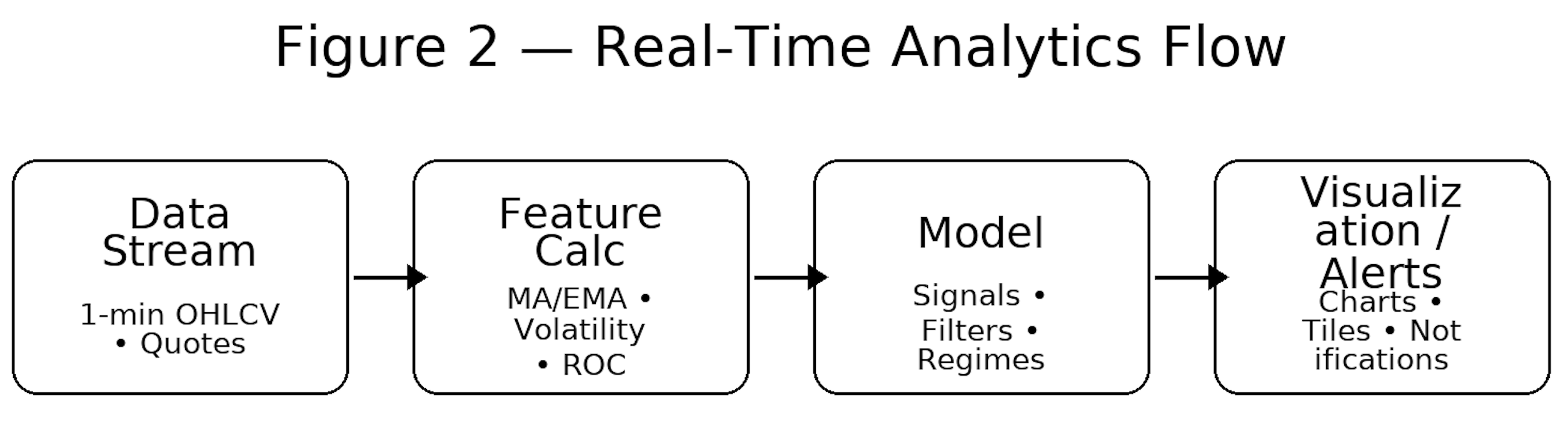
Here's a minimal-average example using Pandas:

df['ma_20'] = df['close'].rolling(20, min_periods=20).mean()

As each new bar lands, your model recalculates features and signals immediately. In quant analysis, real-time data turns historical insight into actionable prediction.

Event-Driven Analysis

Live feeds also detect and react to events: earnings, macro releases, or breaking news often leave signatures (volume/volatility spikes). Event detection systems watch for statistical anomalies — like sudden volume or volatility spikes — that indicate new information hitting the market.

Table 2 — Event-Driven Data Triggers

Event Type	Data Indicator	Response Action
Earnings Release	Sudden volume surge	Alert trader or switch playbook
Fed Announcement	Market-wide volatility jump	Adjust portfolio beta/hedges
Breaking News	Cross-ticker momentum	Pause or execute per rule set

Figure 3 — Real-Time Event Reaction (ASCII: Volume Spike)

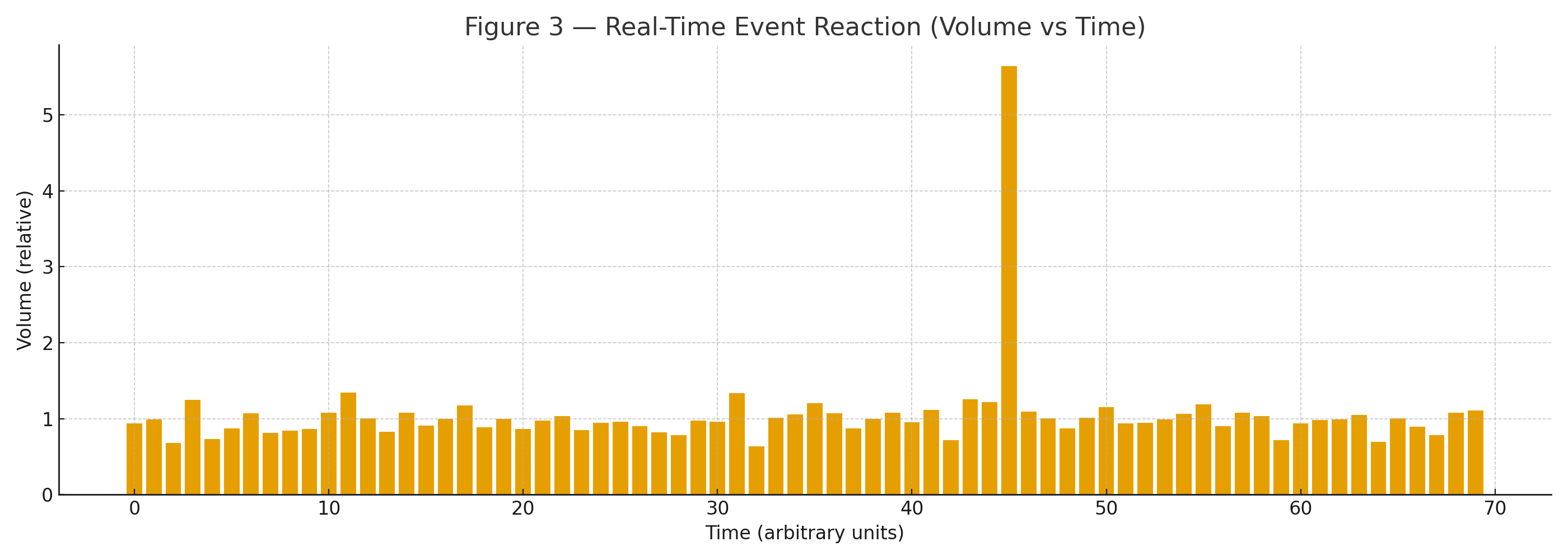
A practical detector compares the last N minutes of volume to a rolling baseline; if the ratio > threshold (e.g., 2.0×), trigger an alert or switch to an “event” mode with different risk and execution rules.

This approach bridges discretionary awareness and automated decision systems.

Integrating Real-Time Data into Models (Python + FMP)

Below is a concise, production-oriented workflow using requests and pandas. Replace api_key with your key.

Figure 4 — Model Integration Flow (API → Python → Strategy)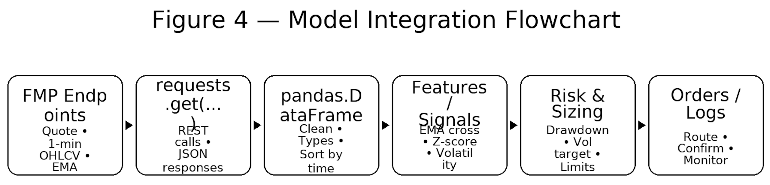

1) Fetch a real-time quote using the FMP Quote API (AAPL)

import requests, pandas as pd

from datetime import datetime

API_KEY = "api_key"

q_url = f"https://financialmodelingprep.com/stable/quote?symbol=AAPL&apikey={API_KEY}"

q = requests.get(q_url, timeout=10).json()[0]

last = q["price"]; vol = q["volume"]

ts = datetime.utcfromtimestamp(q["timestamp"])

print(f"AAPL {last:.2f} @ {ts} UTC | vol={vol:,}")

Use cases: dashboard tiles; latency checks (server timestamp vs. local); regime filters via priceAvg50/200.

2) Pull 1-minute bars and compute intraday features

import math

c_url = f"https://financialmodelingprep.com/stable/historical-chart/1min?symbol=AAPL&apikey={API_KEY}"

bars = requests.get(c_url, timeout=10).json()

df = pd.DataFrame(bars)

df['date'] = pd.to_datetime(df['date'])

df = df.sort_values('date').reset_index(drop=True)

for col in ['open','high','low','close','volume']:

df[col] = pd.to_numeric(df[col], errors='coerce')

df['ret'] = df['close'].pct_change()

df['ema_10'] = df['close'].ewm(span=10, adjust=False).mean()

df['ema_20'] = df['close'].ewm(span=20, adjust=False).mean()

df['z_close'] = (df['close'] - df['ema_20']) / df['ret'].rolling(20).std()

# Annualized intraday volatility proxy (20-min window; ~252 trading days × 390 min/day)

df['vol_20'] = df['ret'].rolling(20).std() * math.sqrt(252 * 390)

Tactics:

• Momentum: go long if ema_10 > ema_20 and ROC positive on rising volume.
• Mean reversion: fade when z_close > +2 (tight stop); cover at mean.
• Volatility-aware sizing: size ∝ 1/vol.

3) Compare to server-side daily EMA (trend filter)

ema_url = ("https://financialmodelingprep.com/stable/technical-indicators/ema"

f"?symbol=AAPL&periodLength=10&timeframe=1day&apikey={API_KEY}")

ema_df = pd.DataFrame(requests.get(ema_url, timeout=10).json())

ema_df['date'] = pd.to_datetime(ema_df['date'])

ema_df = ema_df.sort_values('date')

latest_daily_ema = float(ema_df.iloc[-1]['ema'])

latest_close = float(df.iloc[-1]['close'])

print(f"Daily EMA(10)={latest_daily_ema:.2f} | Last 1m close={latest_close:.2f}")

Blend: only take intraday longs when last price > daily EMA(10).

4) Minimal signal + volatility scaling (illustrative)

# Signal: long when intraday EMA(10) > EMA(20) AND price > daily EMA(10)

df['signal'] = ((df['ema_10'] > df['ema_20']) & (df['close'] > latest_daily_ema)).astype(int)

df['signal'] = df['signal'].shift(1).fillna(0) # act on next bar

# Volatility scaling (toy): cap leverage at 2x

risk_target = 0.01 # 1% daily risk budget

vol_safe = df['vol_20'].replace(0, pd.NA).fillna(method='bfill')

df['pos'] = (risk_target / vol_safe).clip(0, 2.0) * df['signal']

# Naive P&L (ignores fees/slippage/market impact)

df['pnl'] = df['pos'] * df['ret']

5) Event-detection example (volume spike)

# Compare recent volume to rolling baseline

lookback = 20

df['vol_ma'] = df['volume'].rolling(lookback, min_periods=lookback).mean()

df['vol_ratio'] = df['volume'] / df['vol_ma']

df['event_flag'] = (df['vol_ratio'] > 2.0).astype(int) # >2x baseline

if int(df['event_flag'].iloc[-1]) == 1:

print("ALERT: Volume spike detected — switch to event playbook.")

Implementation notes:

• Validate time ordering & gaps; fill/handle missing minutes.Monitor latency (server vs client time); log round-trip.
• Respect rate limits; add retries/backoff.
• Paper-trade before production; add kill switches/circuit breakers.

When these components run together, you have a functional quant prototype — capable of generating and validating live trading signals.

Visualization and Dashboards

Dashboards convert raw ticks into intuition. Once models are generating signals, visualization helps interpret them in real time.

Typical real-time visuals:

• Close with EMA overlays (identify short-term trends)
• Volume bars with anomaly flags
• Volatility panel (rolling σ, ATR)
• Alerts when thresholds breach (e.g., MA cross, breakout)

Figure 5 — Example Real-Time Price Dashboard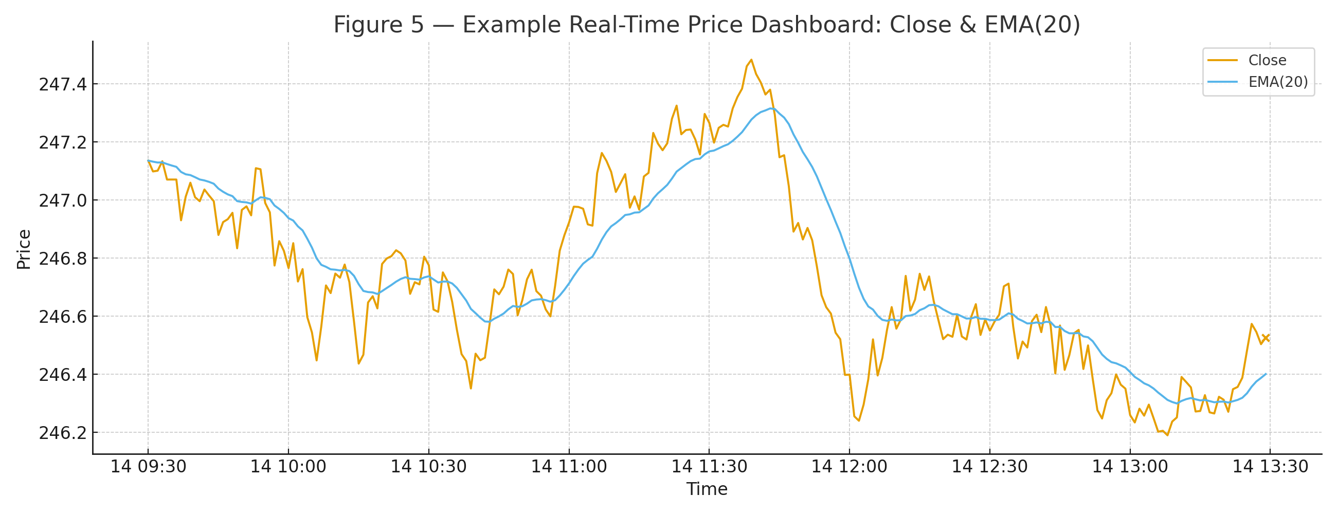

Minimal Matplotlib plot:

import matplotlib.pyplot as plt

ax = df.set_index('date')[['close','ema_20']].plot(figsize=(10,4), linewidth=1.2)

ax.set_title("AAPL — Close vs EMA(20), 1-min")

ax.set_xlabel("Time"); ax.set_ylabel("Price")

plt.tight_layout(); plt.show()

Risk Management and Monitoring

No strategy is complete without safeguards — this section shows how to quantify and react to risk in real time.

Real-time monitoring is risk management in motion. Use live data to enforce limits, reduce size in turbulence, and halt when drawdowns breach rules.

Table 3 — Real-Time Risk Indicators

Indicator	Metric	Update Interval	Use Case
Volatility Index	σ of returns	1m	Adjust leverage/size dynamically
Drawdown	% from running peak	Continuous	Alert risk / auto de-risk

Below are minimal Python examples for tracking volatility and drawdown:

# Rolling volatility (1-min returns)

window = 20

df['vol_20m'] = df['ret'].rolling(window).std()

# Running drawdown on equity curve

df['equity'] = (1 + df['pnl']).cumprod()

df['peak'] = df['equity'].cummax()

df['ddown'] = (df['equity'] / df['peak']) - 1.0

if df['ddown'].iloc[-1] < -0.05: # example: -5% max intraday loss

print("ALERT: Max drawdown exceeded — de-risk now.")

Integrating these alerts into your workflow ensures that capital protection runs as fast as your signal logic.

FAQs

How does FMP provide real-time market data?

FMP delivers millisecond-level updates through REST and WebSocket APIs, combining U.S. and global exchange coverage with low-latency infrastructure.

What is quant analytics?

A data-driven practice that uses statistics, time-series methods, and ML to convert stock market data feeds into signals, risk metrics, and decisions.

How is real-time data used in trading?

It updates features (EMAs, volatility, spreads) and signals the moment a new tick or bar arrives, so orders route with minimal lag.

Can I backtest with real-time feeds?

Backtests use historical data (often the same endpoints but with fixed ranges). After validation, switch to paper/live mode to test with real-time inputs.

What's the difference between live and delayed data?

Live is near-instant; delayed typically lags ~15 minutes. Intraday strategies require live; delayed is fine for end-of-day or long-term investing.