Investors and analysts aim to maximize returns for a given level of risk. The Markowitz model (also known as mean-variance optimization) formalizes this by finding portfolio weights that optimize the risk-return tradeoff.

In practice, this means selecting a mix of assets that maximizes expected return for an allowable level of volatility (risk). We will explain key concepts - efficient portfolios, the efficient frontier, and the variance-covariance matrix - and show how to implement the Markowitz model using Financial Modeling Prep's (FMP) Stock Chart API.

By the end, you'll know how to fetch historical stock data via FMP, compute portfolio returns and risk, and use JavaScript functions to construct an efficient portfolio.

The Markowitz Model and Modern Portfolio Theory

The Markowitz model is the foundation of Modern Portfolio Theory (MPT). In his Nobel-winning 1952 paper, Harry Markowitz showed that by using historical returns and the variances/covariances of assets, one can derive optimal portfolios that offer the highest expected return for a given level of risk.

In other words, no other portfolio can have a higher return without also taking on more risk. This optimization involves calculating each asset's expected return and how it co-moves with every other asset (via the covariance).

The goal is to allocate weights to each asset so that the portfolio's overall expected return is maximized for a target variance (risk) threshold, or conversely, risk is minimized for a target return.

• Mean-Variance Optimization: This method focuses on maximizing return for a given variance (or minimizing variance for a given return). It relies on the inputs of expected returns (means) and the variance-covariance matrix.
• Diversification: By combining assets that are not perfectly correlated, one can reduce portfolio risk without sacrificing return. The Markowitz model quantifies this effect via the covariance terms in the matrix.

In practice, the model is solved as a quadratic optimization: one typically maximizes the Sharpe ratio (return/risk) or minimizes variance subject to return constraints. The result is a series of efficient portfolios.

The Efficient Frontier

The efficient frontier is the set of all efficient portfolios identified by the Markowitz model. Graphically, it is the upward-sloping curve of optimal portfolios on a risk-return plot (risk on x-axis, return on y-axis). Portfolios on this curve offer the maximum expected return for a given risk or equivalently, the minimum risk for a given return.

Below is an abstract illustration of an efficient frontier (for context, not an actual dataset). Each point on the curve is an efficient portfolio for some risk tolerance.

Efficient Frontier graphical representation

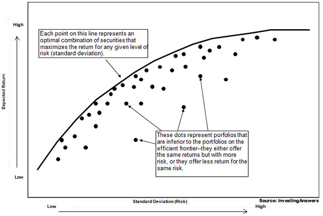
Source: InvestingAnswers

• Definition: No other portfolio exists with a higher expected return at the same level of risk. Portfolios below this frontier are sub-optimal (they leave return on the table for the risk taken).
• Diversification Benefit: The curve is typically convex. Its shape reflects how combining assets with low (or negative) correlations can significantly lower portfolio risk. Interpretation: Risk-averse investors will choose portfolios on the left side of the frontier (lower risk, lower return), while risk-tolerant investors may opt for points on the right (higher risk, higher return).

Calculating Returns and the Variance-Covariance Matrix

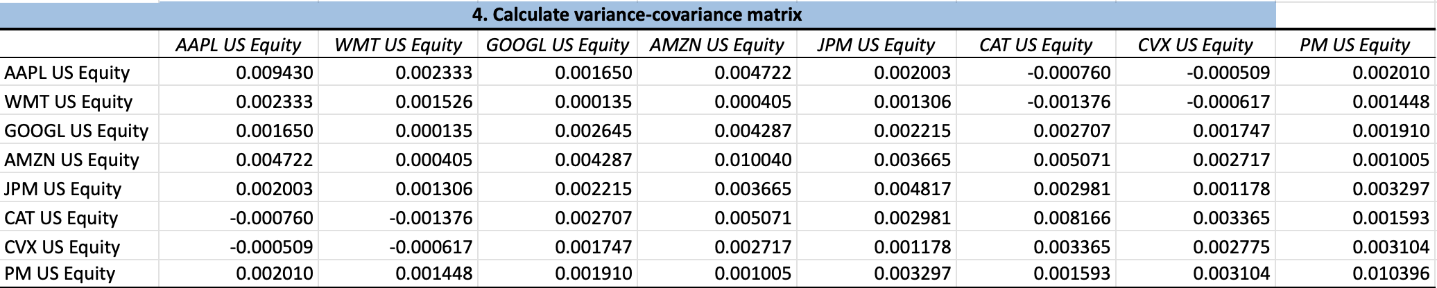
To build and optimize a portfolio, we must calculate asset returns and their statistical relationships. The variance-covariance matrix is central to this. It is a square matrix that holds the variances of each asset's returns on the diagonal and the covariances between every pair of assets off-diagonal. Intuitively, this matrix “generalizes the notion of variance” to multiple assets, capturing how asset returns move together.

The Variance-Covariance Matrix Example

Steps to compute these inputs:

• Historical Price Data: First, gather historical closing prices for each asset in the portfolio (e.g. daily or monthly prices). We will use the FMP Stock Chart API for this.
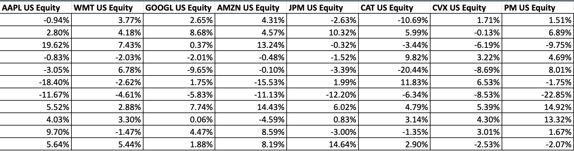
• Daily Returns: Convert prices to returns, typically defined as R_i = (P_i / P_{i-1}) - 1 (or log returns). Returns are calculated for each time step (day) for each asset. These form a returns matrix, where each column is one asset's return series over time.

Stock Daily Returns

Covariance Matrix: With a returns matrix R (dimensions N days × k assets), the covariance matrix Σ (k×k) can be computed as Σ = (1/(N-1)) * (Rᵀ · R) after subtracting mean returns.

In code, for each pair of assets X, Y:

function calculateCovariance(X, Y) { const n = X.length; const meanX = X.reduce((a, b) => a + b, 0) / n; const meanY = Y.reduce((a, b) => a + b, 0) / n; let cov = 0; for (let i = 0; i < n; i++) { cov += (X[i] - meanX) * (Y[i] - meanY); } return cov / (n - 1);}

Using this, you fill the matrix: variances on

Σ[i][i] = calculateCovariance(returns[i], returns[i]), and covariances off-diagonal. For example, a 5-stock portfolio yields a 5×5 covariance matrix.

The covariance matrix encodes portfolio risk. A portfolio's variance is wᵀ Σ w for weight vector w, and the standard deviation (volatility) is the square root. Lower covariances (especially negative) mean the portfolio can achieve a lower overall risk.

Building the Portfolio with FMP Data

Fetch Historical Prices with FMP API

Financial Modeling Prep (FMP) provides an easy way to fetch historical stock prices. The Basic Stock Chart API endpoint returns end-of-day prices and volumes. For example, to get Apple's data:

https://financialmodelingprep.com/stable/historical-price-eod/light?symbol=AAPL&apikey=YOUR_API_KEY

This returns JSON like:

[ {"symbol":"AAPL","date":"2025-11-10","price":269.56,"volume":17890770}, {"symbol":"AAPL","date":"2025-11-07","price":268.47,"volume":48227365}, ...]

Each entry has the date, closing price, and volume. You can replace symbol=AAPL with any ticker, and use your FMP API key.

You can test this endpoint yourself; for example, try fetching another symbol or date range to see the JSON output.

In JavaScript, you might retrieve this data with the fetch API:

async function fetchPrices(symbol) { const apiKey = 'YOUR_API_KEY'; // replace with your FMP key const url = `https://financialmodelingprep.com/stable/historical-price-eod/light?symbol=${symbol}&apikey=${apiKey}`; const resp = await fetch(url); const data = await resp.json(); // Extract just the closing prices return data.map(entry => entry.price);}

Compute Returns and Covariance

After fetching price arrays for each asset, compute daily returns and then form the covariance matrix. For example, suppose we pick five hypothetical symbols (e.g. AAPL, MSFT, AMZN, GOOG, TSLA) and fetch each:

// Example portfolio tickers (hypothetical) const tickers = ['AAPL','MSFT','AMZN','GOOG','TSLA']; // Fetch price series for each ticker (latest N days) - using await or Promise.all let prices = {}; for (let sym of tickers) { prices[sym] = await fetchPrices(sym);} // Compute daily returns for each series function getDailyReturns(priceArr) { let returns = []; for (let i = 1; i < priceArr.length; i++) { returns.push(priceArr[i] / priceArr[i-1] - 1);} return returns;} let returnsData = tickers.map(sym => getDailyReturns(prices[sym])); // Build covariance matrix const numAssets = tickers.length; let covMatrix = Array(numAssets).fill().map(() => Array(numAssets).fill(0)); for (let i = 0; i < numAssets; i++) { for (let j = 0; j < numAssets; j++) { covMatrix[i][j] = calculateCovariance(returnsData[i], returnsData[j]);}}

Now we have each asset's mean return and the covariance matrix Σ of shape 5×5. These are the inputs to the Markowitz optimizer.

Optimizing the Portfolio (Efficient Frontier)

To find the efficient frontier, we solve for weights that optimize risk-return. In practice, one approach is to maximize the Sharpe ratio (return/risk) or solve a quadratic program to minimize variance subject to a target return. The portfolio expected return is R_p = w·μ (dot product of weights with mean returns), and variance is σ_p² = wᵀ Σ w.

In JavaScript, one could implement a simple search or use a numeric library. A sketch of the process:

// Calculate portfolio return function portfolioReturn(weights, meanReturns) { return weights.reduce((sum, w, idx) => sum + w * meanReturns[idx], 0);} // Calculate portfolio variance function portfolioVariance(weights, cov) { let varSum = 0; for (let i = 0; i < weights.length; i++) { for (let j = 0; j < weights.length; j++) { varSum += weights[i] * weights[j] * cov[i][j]; } } return varSum;} // Generate random portfolios and pick best Sharpe ratio function optimizePortfolio(meanReturns, covMatrix, numPortfolios = 100000) { let bestSharpe = -Infinity, bestWeights = null; const riskFreeRate = 0; // assume 0 for simplicity for (let k = 0; k < numPortfolios; k++) { // Random weights that sum to 1 let weights = Array(meanReturns.length).fill().map(() => Math.random()); const total = weights.reduce((a,b) => a+b, 0); weights = weights.map(w => w/total); const ret = portfolioReturn(weights, meanReturns); const vol = Math.sqrt(portfolioVariance(weights, covMatrix)); const sharpe = (ret - riskFreeRate) / vol; if (sharpe > bestSharpe) { bestSharpe = sharpe; bestWeights = weights; } } return { weights: bestWeights, sharpe: bestSharpe };} // Assume meanReturns is an array of each asset's average return const meanReturns = returnsData.map(r => r.reduce((a,b)=>a+b,0)/r.length); const result = optimizePortfolio(meanReturns, covMatrix); console.log("Optimized weights (approx.):", result.weights);

This example shows the idea. In a professional setting, one would use a proper solver (e.g. quadratic programming) to more efficiently trace the efficient frontier. But conceptually, you would vary a target return or maximize Sharpe to get the full frontier of solutions.

Summary of Steps

• Data Retrieval: Fetch historical close prices for each stock via FMP's Stock Chart API
• Return Calculation: Compute daily (or periodic) returns from prices.
• Covariance Matrix: Build the variance-covariance matrix from the returns.
• Optimization: Solve for weights that optimize return/risk. This yields the efficient frontier of portfolios.

Using FMP's APIs ensures your price inputs are accurate and easily accessible. For instance, test the Basic Stock Chart API endpoint with your symbol and key to see real data, then feed that into your Markowitz calculations.

Portfolio Screening and Tools

For investors looking for a guided approach, Stocks2Buy web app offers a stock screener and portfolio builder that leverages these ideas. It lets you filter stocks based on risk factors and automatically constructs a Markowitz-efficient portfolio tailored to your risk appetite. (Note: using Stocks2Buy's features requires your premium FMP API key). This tool is an example of how our models can be embedded in applications: it uses FMP data under the hood to build optimal portfolios.

Efficient Investment Portfolio using the Markowitz Model. Built using the Stocks2Buy app (short sale is allowed)

The Markowitz Model: Optimizing Portfolios for Return and Risk

The Markowitz model provides a rigorous way to build an efficient investment portfolio by balancing return and volatility. Simply fetch historical prices, compute each asset's returns, build the variance-covariance matrix, and solve the mean-variance optimization. The result is the efficient frontier of portfolios, from which investors can choose according to their risk tolerance.

FAQs

What exactly is the Markowitz model?

The Markowitz model is the foundation of Modern Portfolio Theory. It is a mean-variance optimization approach that computes the set of efficient portfolios offering the maximum expected return for each level of risk (volatility). It uses historical returns and their covariance to find the optimal mix of assets.

What is an efficient portfolio?

An efficient portfolio is one that lies on the efficient frontier - meaning no other portfolio has a higher return for the same risk, or a lower risk for the same return. Such portfolios optimally balance risk and reward via diversification.

How do I calculate the variance-covariance matrix?

After computing each asset's returns, the variance-covariance matrix is formed by calculating the covariance between every pair of assets (and variances on the diagonal). You can compute each covariance with the standard formula or a loop over return series (see code above). The matrix summarizes how each asset's return moves relative to the others.

How does the FMP Stock Chart API help build a Markowitz portfolio?

FMP's Stock Chart API provides clean historical price data via a simple REST endpoint. You fetch the price series for each stock in your portfolio, convert them to returns, and then feed those returns into your Markowitz calculations. This ensures you have up-to-date, reliable data for risk and return inputs.

How can I implement this in JavaScript?

Use fetch or similar to call the FMP API endpoint for each symbol (as shown). Then write functions to compute daily returns, mean returns, and the covariance matrix (examples above). Finally, use a numerical method (or simulation) to find portfolio weights that optimize the return/risk ratio. Libraries like math.js or numeric.js can assist with matrix operations if needed.

How can I use my risk appetite with this model?

The efficient frontier allows you to pick a portfolio that matches your risk tolerance. Conservative investors would choose a point on the left side (lower volatility), while aggressive investors can move right on the curve (higher return and risk). Tools like the Stocks2Buy screener let you set risk filters and then automatically apply the Markowitz optimization to suggest a tailored portfolio.