FMP API Trading Edge: Mastering Earnings Surprises and Calendar Data

Earnings days are one of the few times the market is forced to reprice a company in a narrow window. The edge usually is not knowing that earnings matter. It's turning the calendar, estimates, and results into a repeatable pipeline that answers three questions fast: What's coming up, what does the market expect, and how does price typically react when expectations are wrong?

In this article, we'll build that pipeline using FMP's Earnings Calendar and Earnings Report APIs. We'll extract earnings surprise signals, align them with pre and post-earnings price behavior, and turn the output into a practical workflow you can use for screening, alerts, and event-driven trading research.

What you should know about earnings announcements

Earnings announcements are scheduled quarterly events where markets reconcile expectations with reality. In the weeks leading up to the release, analyst models and consensus estimates shape what is already priced in, which is why the same “good” number can still trigger a selloff if it comes in below expectations, or if guidance weakens.

The biggest short-term driver is usually the surprise component. How far actual results deviate from consensus, and in which direction. That gap tends to compress market reaction into a narrow window, with volatility clustering around the announcement as traders reposition and liquidity shifts.

For a trading workflow, the key is not re-learning what earnings are. It's capturing the expectation baseline, measuring the surprise when results land, and then analyzing how price behaves before and after the event so you can screen, time, and size decisions more consistently.

Endpoint Overview

FMP offers the Earnings Calendar API, which allows you to retrieve expected or announced earnings from thousands of companies over a specified period. For this API, you should use:

• api-key: your api key (if you don't have one, you can obtain it by opening a FMP developer account)
• from: the date from which you would like to retrieve the earnings
• To: the date up to which you would like to receive the earnings

The Python pancakes that you will need to import to follow this article are listed below, together with our first basic code that calls this API.

import pandas as pd import requests from datetime import date, timedelta import numpy as np import matplotlib.pyplot as plt import seaborn as sns token = ‘your FMP token' url = f'https://financialmodelingprep.com/stable/earnings-calendar' from_date = '2025-12-01' to_date = '2025-12-31' querystring = {"apikey":token, "from":from_date, "to":to_date} data = requests.get(url, querystring) data = data.json() data

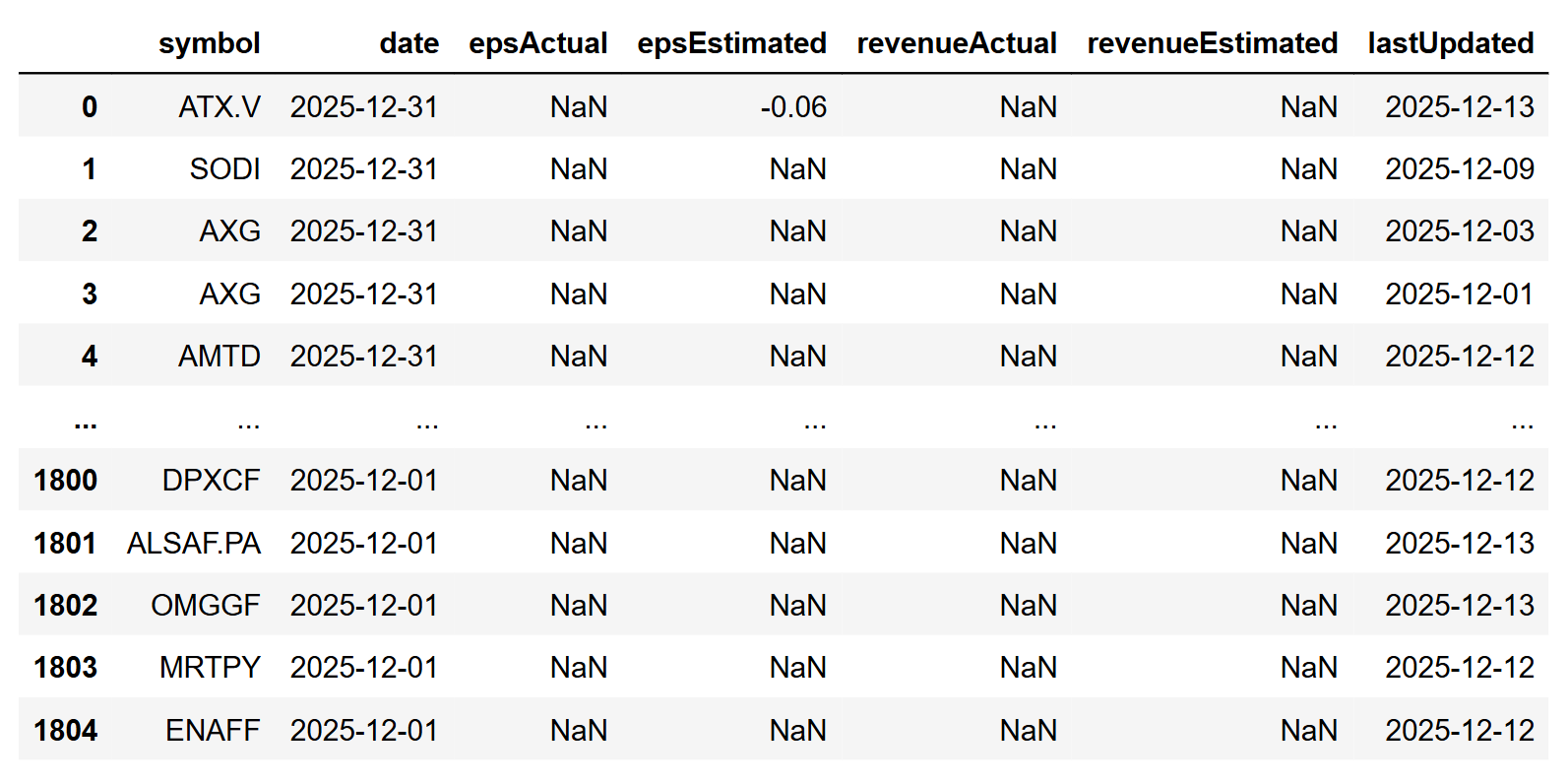
Using the code above, you will get a list of dictionaries for each earning in the requested period. For example:

[{'symbol': 'AXG', 'date': '2025-12-31', 'epsActual': None, 'epsEstimated': None, 'revenueActual': None, 'revenueEstimated': None, 'lastUpdated': '2025-12-03'}, …]

In the above example, you will find:

• symbol: the name of the symbol
• epsActual: Is the value of EPS announced. The API will return None in case of future announcements
• epsEstimated: It is the value of EPS estimated by the analysts. When we get closer to the actual announcement date, this value should be there. You need to know that not all of the shares have enough analysts publishing their expectations, so you should not assume that you will always have an estimated eps.
• revenueActual: like epsActual, those are the revenues announced
• revenueEstimated: like epsEstimated, this is the revenue estimated
• lastUpdated: The date that this entry in FMP's database was last updated. This is handy to understand how old the information is, when the day was that the estimations were published, etc.

Let's see some use cases where you can use this API in the real world:

Get the data and be informed

Assuming you've run the above code, we will transform the response data into a dataframe.

df = pd.DataFrame(data)

Some useful filters to view the results include checking which of your earnings data have already been announced.

df[df['epsActual'].notna()]

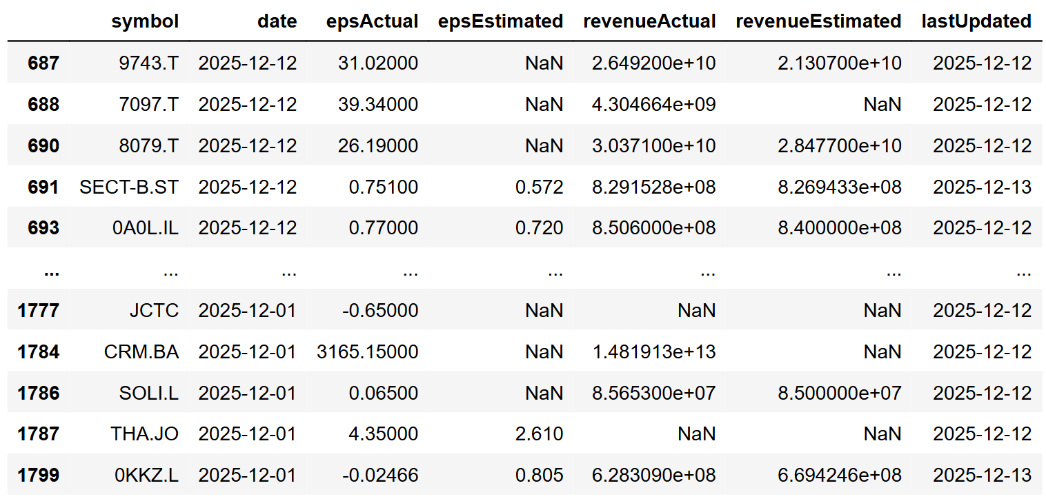
With a quick glance, you can identify which companies have announced their earnings and for which an estimated eps has been published.

Another handy filter is to see the earnings that have not been published yet, and an estimation exists.

df[df['epsEstimated'].notna() & df['epsActual'].isna()]

Using the above knowledge, we can quickly create our first example. By running the code below, you can see the upcoming week's earnings to be announced and the published estimation. Remember, the nearer we are to the announcement date, the better your chances of seeing an estimation.

today = date.today() tomorrow = today + timedelta(days=1) after_one_week = today + timedelta(weeks=1) url = f'https://financialmodelingprep.com/stable/earnings-calendar' querystring = {"apikey":token, "from":tomorrow, "to":after_one_week} data = requests.get(url, querystring) data = data.json() df = pd.DataFrame(data) df = df[df['epsEstimated'].notna() & df['epsActual'].isna()] # sort values by date df = df.sort_values(by='epsEstimated', ascending=False) df[['date','symbol','epsEstimated']]

The code filters for earnings that have a published estimate but no actual figure, sorting them by the largest expected EPS and displaying only the date, symbol, and estimated earnings per share. This matters because surprise-driven volatility is only meaningful when expectations are defined. Without an estimate baseline, you cannot quantify a surprise or build a consistent pre-earnings watchlist around it.

At the time of executing the above code, we got the following results:

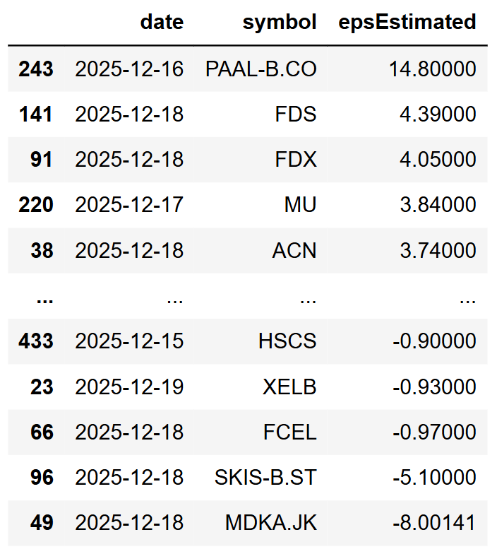
It is important to clarify that the EPS is displayed in the trading currency of the stock. For example, the first symbol PAAL-B.CO is in DKK, not USD, while FedEx (FDX) or Micron Technology (MU) are in USD.

Visualising Historical Earnings

After you obtain the above information, your next step might be to investigate the historical earnings of a specific share. For this, another important FMP API is the FMP's Earnings Report API, where you can access the same information as the previous API, but for a specific share.

symbol = 'FDX' url = 'https://financialmodelingprep.com/stable/earnings' querystring = {"apikey": token, "symbol": symbol} data = requests.get(url, querystring) data = data.json() df = pd.DataFrame(data) df = df[df['epsActual'].notna()].copy() df = df.sort_values(by='date') df.plot(x='date', y='epsActual', figsize=(12, 5), title=f"{symbol} EPS Actual")

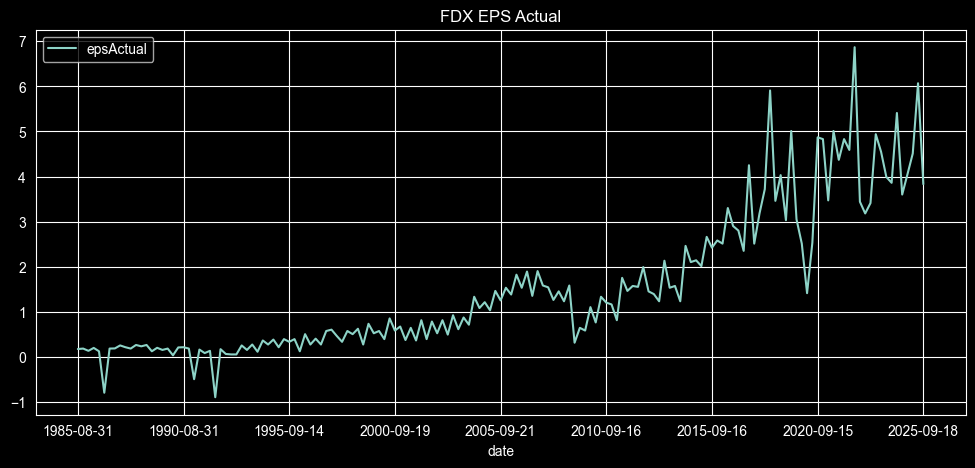
You can observe that we have data spanning approximately 40 years, and we can plot the earnings per share for that period, illustrating the development of the revenue. Note that by changing the symbol variable to your preferred one, the code will generate a plot for the share you are interested in.

With some extra Python code, we can also plot the element of surprise.

pct_surpized = 0.10 df['date'] = pd.to_datetime(df['date'], errors='coerce') # [web:19] df['epsActual'] = pd.to_numeric(df['epsActual'], errors='coerce') df['epsEstimated'] = pd.to_numeric(df['epsEstimated'], errors='coerce') valid_est = df['epsEstimated'].notna() is_green = valid_est & (df['epsActual'] > (df['epsEstimated'] * (1 + pct_surpized))) is_red = valid_est & (df['epsActual'] < (df['epsEstimated'] * (1 - pct_surpized))) bar_colors = np.where(is_green, 'green', np.where(is_red, 'red', 'none')) edge_colors = np.where(is_green, 'green', np.where(is_red, 'red', 'grey')) x = np.arange(len(df)) w = 0.42 plt.figure(figsize=(12, 5)) plt.bar(x + w / 2, df['epsActual'], width=w, color=bar_colors, edgecolor=edge_colors, linewidth=0.5, label='epsActual') plt.title(f"{symbol} EPS Actual") plt.xlabel("Date") plt.ylabel("EPS") years = df['date'].dt.year first_idx_per_year = years.groupby(years).transform('idxmin') # [web:16] mask_year_change = df.index == first_idx_per_year mask_5y = (years % 5 == 0) final_mask = mask_year_change & mask_5y tick_positions = x[final_mask] tick_labels = years[final_mask].astype(str) plt.xticks(tick_positions, tick_labels, rotation=45, ha='right') # [web:3][web:9] plt.legend() plt.grid(axis='y', alpha=0.25) plt.tight_layout() plt.show()

The above code calculates the element of surprise in the announcement and plots in green the announcements where the actuals exceeded the estimates, in red the cases where the actuals were less than the estimates, and with outlined empty bars when analysts estimated correctly. The element of surprise is expressed as a percentage with the variable pct_surprised set at 10% (0.10), which means the actual was more than 10% above or below the estimate. You can adjust this threshold to control sensitivity. In practice, it becomes a simple filter for separating noise from meaningful earnings reactions, and it can be used to select events for backtesting or to trigger alerts when a print crosses a predefined surprise level. With the 10% setting, the plot looks like the one below.

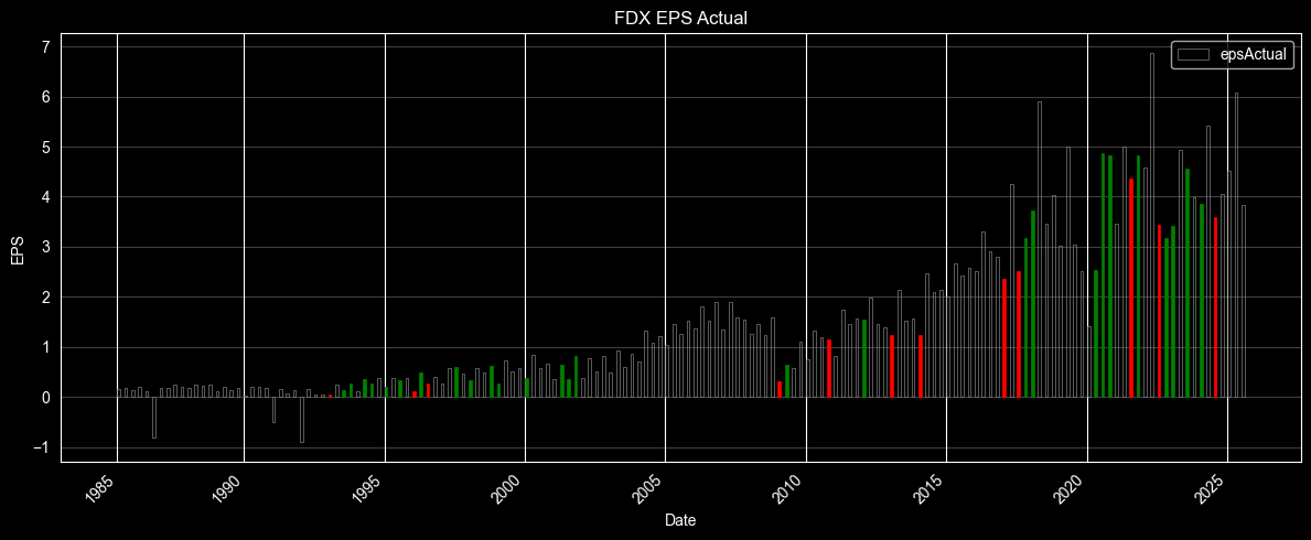
We can see that for FedEx, in recent years the estimates were either accurate or the surprise was positive, with a few negative surprises when earnings disappointed investors.

Let's add the prices

Another opportunity to gain more detailed insights would be to include the historical prices of the stock and examine the correlations between earnings announcements and price fluctuations around the announcement date.

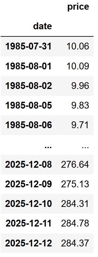
First, we will obtain the daily stock's prices. The code will attempt to retrieve prices from the earliest published earnings using the relevant FMP endpoint and will retain only the adjusted closing price.

url = f'https://financialmodelingprep.com/api/v3/historical-price-full/{symbol}' min_ts = (df['date'].min() - pd.DateOffset(months=1)).strftime('%Y-%m-%d') querystring = {"apikey":token, "from": min_ts} resp = requests.get(url, querystring).json() df_prices = pd.DataFrame(resp['historical'])[['date', 'adjClose']] df_prices['date'] = pd.to_datetime(df_prices['date']) df_prices.set_index('date', inplace=True) df_prices.rename(columns={'adjClose':'price'}, inplace=True) df_prices = df_prices.sort_index(ascending=True) df_prices

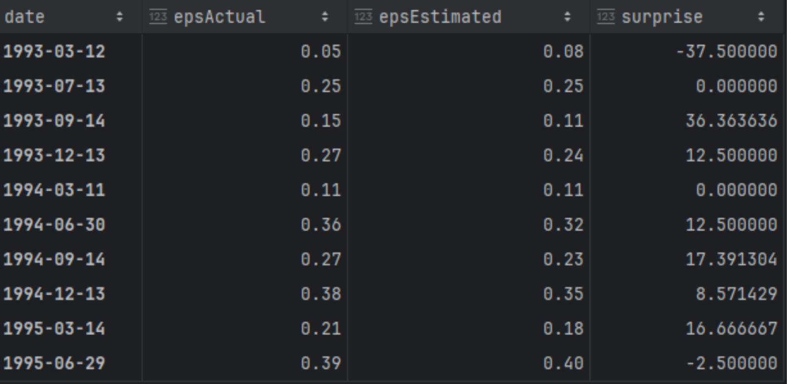
Additionally, we will create a dataframe named df_eps where we will store the actual, the estimated figures, and also calculate the surprise as a percentage.

df_eps = df[['date','epsActual','epsEstimated']] df_eps['surprise'] = ((df_eps['epsActual'] - df_eps['epsEstimated'])/df_eps['epsEstimated']) * 100 df_eps['date'] = pd.to_datetime(df_eps['date']) df_eps.set_index('date', inplace=True) df_eps

Now that we have our EPS and prices dataframes, let's begin calculating some columns and metrics needed for the correlation analysis.

First, we will add to our EPS dataframe the stock price on the day of the announcement, as well as 5 days before and 5 days after.

# ensure datetime index and sorted df_eps.index = pd.to_datetime(df_eps.index) df_prices.index = pd.to_datetime(df_prices.index) df_prices = df_prices.sort_index() days_diff = 5 price = df_prices['price'] df_eps['price_0d'] = price.reindex(df_eps.index, method='ffill') idx_before = df_eps.index - pd.Timedelta(days=days_diff) df_eps[f'price_-{days_diff}d'] = price.reindex(idx_before, method='ffill').to_numpy() idx_after = df_eps.index + pd.Timedelta(days=days_diff) df_eps[f'price_+{days_diff}d'] = price.reindex(idx_after, method='ffill').to_numpy()

And after we obtain those prices, we will calculate the following:

• the percentage between the previous actual earnings and the estimated, to capture if the expected earnings will be more than the previous ones
• the same as the above, but this time comparing actual to previous actual earnings, to capture the actual growth
• the price difference between the price on the day of announcement, compared to the price that was 5 days before
• the price difference between the price on the day of the announcement, compared to the price 5 days after

# previous EPS actual df_eps['epsActual_prev'] = df_eps['epsActual'].shift(1) df_eps['pct_est_vs_prev_actual'] = ( (df_eps['epsEstimated'] - df_eps['epsActual_prev']) / df_eps['epsActual_prev'] ) df_eps['pct_actual_vs_prev_actual'] = ( (df_eps['epsActual'] - df_eps['epsActual_prev']) / df_eps['epsActual_prev'] ) df_eps[f'pct_price_0d_vs_-{days_diff}d'] = ( (df_eps['price_0d'] - df_eps[f'price_-{days_diff}d']) / df_eps[f'price_-{days_diff}d'] ) df_eps[f'pct_price_+{days_diff}d_vs_0d'] = ( (df_eps[f'price_+{days_diff}d'] - df_eps['price_0d']) / df_eps['price_0d'] ) cols = [ 'pct_est_vs_prev_actual', 'pct_actual_vs_prev_actual', f'pct_price_0d_vs_-{days_diff}d', f'pct_price_+{days_diff}d_vs_0d', ] df_eps[cols] = df_eps[cols] * 100

Now we can plot a correlation heatmap.

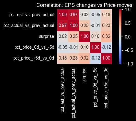
Correlation gives you a quick sense of direction, but it rarely tells a clean story around earnings. Price moves are reacting to more than just the EPS print. Guidance, commentary, positioning, and even how crowded the trade is can matter just as much. With that in mind, a couple of relationships are still worth noting.

• The element of surprise vs the price move after the announcement shows a 0.32 correlation. It's not strong, but it does suggest that larger surprises tend to come with larger post-earnings moves, which is the kind of relationship you can sanity-check before building any earnings-driven screen.
• There's also a slight negative correlation between the returns before and after the announcement (-0.12). That hints at pre-earnings positioning and reversal behavior in some cases. It's a reminder that you can't treat surprise as a standalone signal. If you plan to use it, you'll want to test it in combination with context like pre-earnings drift, direction of the move, and how quickly the market digests the information.

AI-Powered Analysis: Extracting Trading Insights from Earnings Transcripts

In today's world, AI is at the forefront of traders' discussions, whether for investing in AI companies or using AI to identify investment opportunities.

Another useful FMP's API is the Earnings Transcript API. After the official earnings announcement, the CEO typically joins a call with analysts and investors to discuss the results and the company's strategy. By using this API, we can obtain the transcript and input it into our preferred AI model to generate insights, eliminating the need to read the entire document.

symbol = 'FDX' year = 2026 quarter = 1 url = 'https://financialmodelingprep.com/stable/earning-call-transcript' querystring = {"apikey": token, "symbol": symbol, "year": year, "quarter": quarter} data = requests.get(url, querystring) data = data.json() pd.Series([data[0]['content']]).to_clipboard(index=False, header=False) data[0]['content']

Since those calls are related to strategy, they are documented for future reference with dates in the future. In our case, we will obtain the 2026 and first quarter transcripts for FedEx.. Note that the code also practically copies the transcript into our clipboard, allowing us to easily paste it into an AI model. Use AI here as a fast triage layer to pull out themes and questions worth investigating, but still treat the output as unverified since models can miss context, reflect bias, or hallucinate details, so you should validate anything important against the original transcript.

In our example, we will use Perplexity. We will prompt it “Give us in 5 bullet points, the most important parts of this transcript that is expected to effect the price of the stock for the next 6 months” and then we will paste the transcript

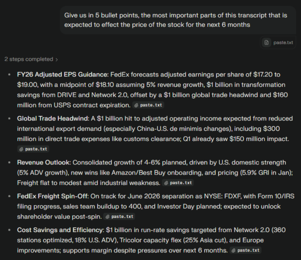
This provided us with the five most important points discussed during the call within seconds. Depending on the responses, we can continue our discussion with the model, for example by asking it about risks.

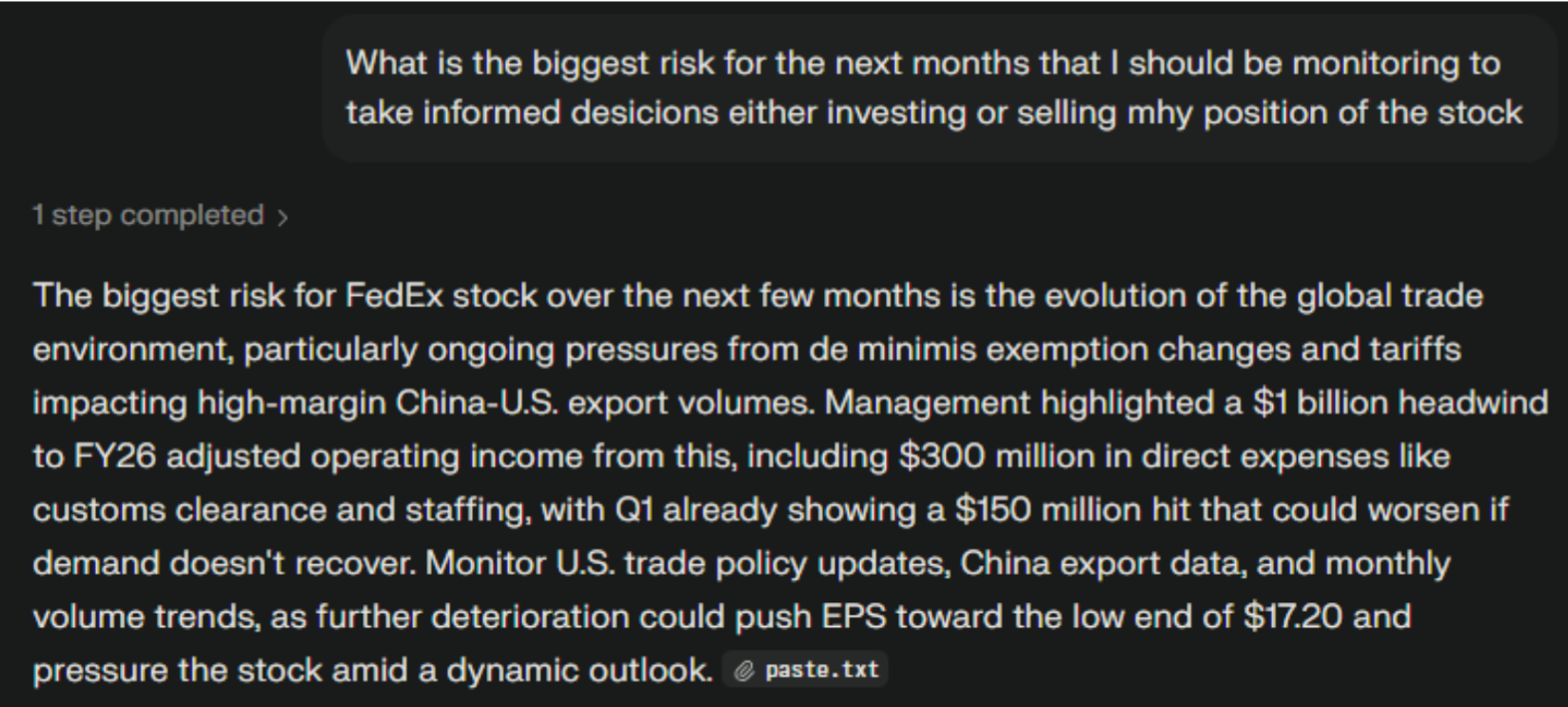
We can see that the model is informing us that FedEx is connected to the evolution of global trade, and monitoring the high-margin China-US exports should continue, as they are likely to affect the company's revenues.

Final Thoughts

The main takeaway here is the workflow. You start with the calendar to see what's coming up, filter for cases where estimates exist, then measure the surprise once actuals print. After that, you line the event up with price action to understand what tends to happen before and after earnings. The transcript step is there to add context. It helps you quickly spot what management focused on and what risks or themes were repeated.

If you keep this flow consistent, it becomes a solid template you can reuse across tickers and quarters. You can plug it into a simple watchlist, build alerts for large surprises, or expand it into a backtesting dataset if you want to study post-earnings moves more systematically.