A Form 13F is a regulatory disclosure, not a portfolio report. It lists long positions in certain U.S.-listed securities held by institutional investment managers at the end of each calendar quarter. The filing includes issuer names, CUSIPs, share counts, and reported market values, all presented in a standardized format. Analysts typically source and standardize this disclosure data through platforms like Financial Modeling Prep (FMP) when they want to turn filings into clean, queryable datasets.

This structure is intentional. It allows regulators and the public to see where institutional capital is allocated at a specific point in time, using consistent definitions across managers. The filing answers one narrow question: what long equity positions were reported at quarter's end.

What the Data Reliably Reveals

Within that scope, 13F data is dependable. It shows position size at the security level, relative concentration within the disclosed portfolio, and changes in reported holdings across quarters. When aggregated, it allows comparison across managers and identification of overlapping exposure.

Used correctly, this data supports descriptive analysis. Analysts can observe where reported capital clusters, which positions persist over time, and how disclosed holdings evolve from one quarter to the next. These insights come from the consistency of the disclosure format, not from any implied intent behind the positions.

Descriptive in this context does not mean actionable on its own; it means the data provides context and structure that must be combined with other signals before informing decisions.

What the Filing Does Not Attempt to Explain

A 13F does not describe how or why a position exists. It does not indicate holding period, conviction, or risk contribution. It does not show whether a position is hedged, paired, or offset elsewhere in the portfolio.

The filing records inventory, not strategy. Confusing the two is the most common source of misinterpretation. Understanding what the form is built to show, and where it deliberately stops, is the foundation for any disciplined use of 13F data.

The Built-in Lag Problem

One of the most misunderstood aspects of Form 13F data is timing. The information disclosed is accurate as of a specific date, but it is never contemporaneous with how portfolios actually evolve in the market. Understanding this lag is critical, because many common misuses of 13F filings stem from treating delayed disclosures as if they reflected live positioning.

The lag shows up in two distinct ways: when holdings are measured, and when those measurements become public.

Quarter-End Snapshots, Not Live Positioning

Form 13F filings report holdings as of the last day of each calendar quarter. That date matters more than the filing itself. Every position listed reflects exposure at a single point in time, not an ongoing or current portfolio state.

From an analytical standpoint, this means the data is historical the moment it exists. Any trades executed after quarter end—reductions, additions, exits—are invisible to the filing. Treating a 13F as a view of “what a manager owns now” misrepresents what the disclosure actually captures.

The Disclosure Delay

Public access to a 13F filing occurs weeks after the quarter closes. During that gap, markets move, earnings are released, and portfolios adjust. By the time the data becomes available, it may already be several market events behind.

This delay does not invalidate the data. It defines how it should be used. A 13F is a backward-looking record, not a real-time signal. FMP's walkthrough on extracting 13F data also emphasizes this delay constraint and shows how to use filings as a long-horizon signal layer rather than a real-time trading feed. Any analysis that assumes immediacy introduces error.

Keeping Market Context Aligned

Because of the lag, market data must be aligned to the same reporting window as the filing. Comparing quarter-end holdings to current prices blends two different timeframes and creates misleading conclusions.

Effective analysis anchors interpretation to the reporting period itself. Prices, returns, and events should be evaluated within the same quarter the holdings represent. This preserves consistency and keeps conclusions grounded in what the disclosure actually reports.

The lag is not a flaw. It is a structural constraint. Recognizing it early prevents overreach and keeps 13F analysis within its intended boundaries.

What 13F Cannot Show by Design

Even when timing is handled correctly, Form 13F filings still provide only a partial view of institutional portfolios. The limits are not accidental or due to incomplete reporting. They are structural boundaries defined by what the regulation requires managers to disclose.

Understanding these boundaries is essential. Many of the most common misinterpretations of 13F data come from assuming the filing represents a complete or risk-adjusted portfolio view, when it does not.

Missing Exposures and Incomplete Portfolios

Form 13F filings report only long positions in certain U.S.-listed equity securities. Everything else is excluded by definition. Short positions, derivatives, bonds, commodities, private investments, and most non-U.S. holdings never appear in the disclosure.

As a result, the filing represents only a slice of an institutional portfolio. It shows reported long exposure, not total exposure. Any analysis that treats a 13F as a complete portfolio view overstates what the data actually contains.

Gross Exposure Versus Economic Exposure

Because short positions and hedges are not disclosed, a reported long position does not necessarily reflect net risk. A large holding may be fully or partially offset elsewhere in the portfolio through derivatives or paired trades.

This distinction matters. The filing shows gross positions, not economic exposure. Without visibility into offsets, the data cannot reveal how much risk the manager is actually taking on a given security or sector.

No Visibility into Intent or Time Horizon

A 13F does not explain why a position exists. It does not distinguish between a long-term investment, a temporary trade, an index-related holding, or a mandate-driven allocation.

Holding period, conviction, and portfolio role remain unknown. A position that appears stable across quarters may reflect structural exposure rather than active decision-making. A sharp change may reflect rebalancing rather than a change in view.

These omissions are not gaps in reporting. They are deliberate boundaries. Understanding them prevents analysts from attributing strategy, conviction, or risk posture to data that was never meant to convey those signals.

Turning a 13F Filing Into a Usable Dataset (with Python)

This section is not intended to serve as a complete 13F analysis guide. Instead, it illustrates how the structural constraints discussed earlier—timing, disclosure scope, and reporting consistency—translate into a practical data shape that supports disciplined analysis.

The example focuses on structure and alignment rather than exhaustive implementation. For full workflows and broader context on extracting and interpreting institutional ownership data, see FMP's Mastering 13F Filings overview and the How to Gain Investment Insights from Form 13F Using FMP's Filings Extract API tutorial, and consult FMP's Form 13F APIs dataset page for endpoint details.

The first practical step is to remove guesswork around timing. Instead of hardcoding a year and quarter, the workflow queries the list of available filing periods for a manager using the Form 13F Filings Dates API and selects the most recent completed quarter. This step is shown to demonstrate alignment discipline, not to prescribe a specific implementation pattern. This guarantees the dataset reflects what is actually on file, not what we assume should be there.

This step matters because every downstream metric—weights, concentration, changes—depends on anchoring analysis to the correct reporting window. When you scale this workflow across many managers, request volume and endpoint access depend on the plan, so it helps to align your pipeline with FMP pricing plans.

Pulling Reported Holdings

Once the period is fixed, the holdings for that quarter can be retrieved at the security level. The script pulls position-level rows through the Filings Extract API, which returns issuer, CUSIP, shares, and reported value in a structured format. Each row represents a disclosed long position and includes issuer name, CUSIP, share count, and reported value.

Reported values in 13F filings are expressed in thousands of dollars. Treating them as raw dollars inflates portfolio size and distorts weights. Normalizing this correctly is essential before any interpretation.

At this point, the filing stops being a document and becomes a structured dataset.

Computing Weights and Concentration

Raw holdings lists describe inventory, not structure. To understand what the filing reveals, positions need to be normalized within the disclosed portfolio.

Weights convert reported values into relative exposure. From there, basic concentration metrics become meaningful. Top holdings show dominance. Aggregate weights for the top five or ten positions indicate focus. A simple concentration index summarizes how clustered the disclosed capital is.

These calculations do not infer intent. They describe what is visible in the filing, nothing more. If you want to extend this into an automated research workflow, FMP's guide on building a 13F filing analyzer shows how to layer extraction, normalization, and interpretation without over-claiming what filings can prove.

Python Implementation

import os import requests import pandas as pd from requests.adapters import HTTPAdapter from urllib3.util.retry import Retry BASE_URL = "https://financialmodelingprep.com/stable" API_KEY = os.getenv("FMP_API_KEY") # or set directly def get_session(): session = requests.Session() retry = Retry( total=4, backoff_factor=0.5, status_forcelist=[429, 500, 502, 503, 504], allowed_methods=["GET"], ) session.mount("https://", HTTPAdapter(max_retries=retry)) return session def fetch_13f_periods(cik: str): url = f"{BASE_URL}/institutional-ownership/dates" params = {"cik": cik, "apikey": API_KEY} with get_session() as s: r = s.get(url, params=params, timeout=20) r.raise_for_status() return r.json() def pick_latest_period(periods): if not periods: raise ValueError("No 13F filing periods available.") latest = max(periods, key=lambda p: (int(p["year"]), int(p["quarter"]))) return int(latest["year"]), int(latest["quarter"]) def fetch_13f_holdings(cik: str, year: int, quarter: int): url = f"{BASE_URL}/institutional-ownership/extract" params = { "cik": cik, "year": year, "quarter": quarter, "apikey": API_KEY } with get_session() as s: r = s.get(url, params=params, timeout=20) r.raise_for_status() return r.json() def build_holdings_table(holdings: list): df = pd.DataFrame(holdings) # Rename only if columns exist rename_map = { "nameOfIssuer": "issuer", "cusip": "cusip", "value": "value_usd_thousands", "sshPrnamt": "shares", } df = df.rename(columns={k: v for k, v in rename_map.items() if k in df.columns}) # Select available columns safely desired_cols = ["issuer", "cusip", "value_usd_thousands", "shares"] available_cols = [c for c in desired_cols if c in df.columns] df = df[available_cols] # Ensure numeric fields if "value_usd_thousands" in df.columns: df["value_usd_thousands"] = pd.to_numeric( df["value_usd_thousands"], errors="coerce" ) total_value = df["value_usd_thousands"].sum(skipna=True) df["weight_pct"] = (df["value_usd_thousands"] / total_value) * 100 df = df.sort_values("value_usd_thousands", ascending=False) # Concentration metrics top5_weight = df.head(5)["weight_pct"].sum() top10_weight = df.head(10)["weight_pct"].sum() weights = (df["weight_pct"] / 100).fillna(0) hhi = (weights ** 2).sum() summary = { "total_value_usd_thousands": float(total_value), "top5_weight_pct": float(top5_weight), "top10_weight_pct": float(top10_weight), "hhi": float(hhi), } return df, summary if __name__ == "__main__": cik = "0001067983" # example CIK periods = fetch_13f_periods(cik) year, quarter = pick_latest_period(periods) holdings = fetch_13f_holdings(cik, year, quarter) table, stats = build_holdings_table(holdings) print(f"Latest filing: {year} Q{quarter}") print("Summary:", stats) print("\nTop 10 positions:") print(table.head(10).to_string(index=False))

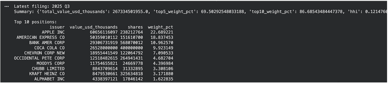
Interpretation of The Output

The output reflects the most recent available Form 13F filing, corresponding to 2025 Q3. It summarizes the disclosed long equity positions reported at quarter end and presents both portfolio-level concentration metrics and position-level detail.

The concentration summary indicates that the disclosed portfolio is highly concentrated. The top five positions account for approximately 69.5% of total reported value, while the top ten positions represent approximately 86.7%. This distribution shows that reported exposure is dominated by a small number of holdings rather than evenly distributed across the filing.

The position table ranks securities by reported market value and displays their relative weight within the disclosed portfolio. Apple Inc. is the largest reported holding, representing approximately 22.7% of disclosed value. It is followed by American Express and Bank of America, which together contribute a substantial share of the remaining exposure. Subsequent positions decline progressively in relative weight.

This output describes the structure of reported long holdings at a specific reporting date. It identifies concentration and dominant positions within the disclosure but does not provide insight into portfolio intent, hedging activity, or net exposure. The information should therefore be interpreted as a descriptive snapshot of reported holdings rather than a representation of complete portfolio strategy.

Multi-Quarter Changes That Actually Mean Something

Single-quarter snapshots describe structure, but they do not explain behavior. To understand how reported holdings evolve, 13F data needs to be observed across multiple filing periods. Changes over time provide context that a single disclosure cannot.

Tracking Position Persistence and Exits

Comparing the same positions across consecutive quarters helps distinguish persistent holdings from temporary ones. Positions that appear consistently across filings suggest ongoing exposure at the reporting dates. Positions that disappear or reappear intermittently indicate turnover rather than sustained presence.

This approach avoids attributing significance to positions that appear large in one quarter but have no continuity in subsequent filings.

Identifying Meaningful Share Changes

Quarter-over-quarter changes in reported share counts provide a clearer signal than changes in reported value alone. Value can fluctuate due to market price movements, while share changes reflect actual adjustments in reported position size.

Focusing on material increases or reductions in shares helps identify where reported exposure has shifted meaningfully between reporting periods, without conflating trading activity with market volatility.

Avoiding Single-Quarter Misreads

Isolated changes can be misleading. A large increase in one quarter may reverse in the next. Multi-quarter comparisons reduce this noise and help separate structural changes from short-term adjustments.

Used this way, 13F data supports trend observation rather than inference. The emphasis remains on what the disclosures show consistently over time, not on speculative interpretation of individual filings.

Python Code: Tracking Quarter-Over-Quarter Share Changes

import os import requests import pandas as pd from requests.adapters import HTTPAdapter from urllib3.util.retry import Retry BASE_URL = "https://financialmodelingprep.com/stable" API_KEY = os.getenv("FMP_API_KEY") # or set directly def get_session(): s = requests.Session() retry = Retry( total=4, backoff_factor=0.5, status_forcelist=[429, 500, 502, 503, 504], allowed_methods=["GET"], ) s.mount("https://", HTTPAdapter(max_retries=retry)) return s def fetch_13f_holdings_df(cik: str, year: int, quarter: int) -> pd.DataFrame: url = f"{BASE_URL}/institutional-ownership/extract" params = {"cik": cik, "year": year, "quarter": quarter, "apikey": API_KEY} with get_session() as s: r = s.get(url, params=params, timeout=20) r.raise_for_status() data = r.json() return pd.DataFrame(data) def normalize_holdings(df: pd.DataFrame) -> pd.DataFrame: # Keep original fields if present; also create standard names. rename_map = { "nameOfIssuer": "issuer", "sshPrnamt": "shares", "value": "value_usd_thousands", "titleOfClass": "class_title", "cusip": "cusip", "symbol": "symbol", } df = df.rename(columns={k: v for k, v in rename_map.items() if k in df.columns}).copy() # Ensure numeric if "shares" in df.columns: df["shares"] = pd.to_numeric(df["shares"], errors="coerce") if "value_usd_thousands" in df.columns: df["value_usd_thousands"] = pd.to_numeric(df["value_usd_thousands"], errors="coerce") return df def choose_join_key(cur: pd.DataFrame, prev: pd.DataFrame) -> str: """ Prefer a stable identifier that exists in BOTH quarters. """ candidates = ["cusip", "symbol"] for c in candidates: if c in cur.columns and c in prev.columns and cur[c].notna().any() and prev[c].notna().any(): return c # Fallback: composite key from issuer + class title (last resort) if "issuer" in cur.columns and "issuer" in prev.columns: cur["join_key"] = cur["issuer"].fillna("").astype(str).str.strip() prev["join_key"] = prev["issuer"].fillna("").astype(str).str.strip() if "class_title" in cur.columns and "class_title" in prev.columns: cur["join_key"] = cur["join_key"] + " | " + cur["class_title"].fillna("").astype(str).str.strip() prev["join_key"] = prev["join_key"] + " | " + prev["class_title"].fillna("").astype(str).str.strip() return "join_key" raise ValueError("No usable join key found. The filing data is missing both CUSIP/Symbol and issuer fields.") def compute_qoq_changes(cik: str, current: tuple, previous: tuple) -> pd.DataFrame: cy, cq = current py, pq = previous cur = normalize_holdings(fetch_13f_holdings_df(cik, cy, cq)) prev = normalize_holdings(fetch_13f_holdings_df(cik, py, pq)) join_col = choose_join_key(cur, prev) # Select a minimal set of columns safely cur_cols = [join_col] + [c for c in ["issuer", "shares", "value_usd_thousands"] if c in cur.columns] prev_cols = [join_col] + [c for c in ["issuer", "shares", "value_usd_thousands"] if c in prev.columns] cur = cur[cur_cols].copy() prev = prev[prev_cols].copy() merged = cur.merge(prev, on=join_col, how="outer", suffixes=("_current", "_previous")) # Choose issuer label: prefer current if "issuer_current" in merged.columns or "issuer_previous" in merged.columns: merged["issuer"] = merged.get("issuer_current").fillna(merged.get("issuer_previous")) # shares: missing => 0 (new or exited) merged["shares_current"] = pd.to_numeric(merged.get("shares_current"), errors="coerce").fillna(0) merged["shares_previous"] = pd.to_numeric(merged.get("shares_previous"), errors="coerce").fillna(0) merged["share_change"] = merged["shares_current"] - merged["shares_previous"] # optional value change (kept if available) if "value_usd_thousands_current" in merged.columns or "value_usd_thousands_previous" in merged.columns: merged["value_usd_thousands_current"] = pd.to_numeric( merged.get("value_usd_thousands_current"), errors="coerce" ).fillna(0) merged["value_usd_thousands_previous"] = pd.to_numeric( merged.get("value_usd_thousands_previous"), errors="coerce" ).fillna(0) merged["value_change_usd_thousands"] = ( merged["value_usd_thousands_current"] - merged["value_usd_thousands_previous"] ) out_cols = [join_col] if "issuer" in merged.columns: out_cols.insert(0, "issuer") out_cols += ["shares_previous", "shares_current", "share_change"] if "value_change_usd_thousands" in merged.columns: out_cols.append("value_change_usd_thousands") merged = merged[out_cols].copy() return merged.sort_values("share_change", ascending=False).reset_index(drop=True), join_col if __name__ == "__main__": cik = "0001067983" # Example: compare two consecutive quarters changes, join_used = compute_qoq_changes(cik, current=(2025, 3), previous=(2025, 2)) print(f"Join key used: {join_used}") print("\nTop 10 increases in reported shares:") print(changes.head(10).to_string(index=False)) print("\nTop 10 reductions in reported shares:") print(changes.tail(10).sort_values("share_change").to_string(index=False))

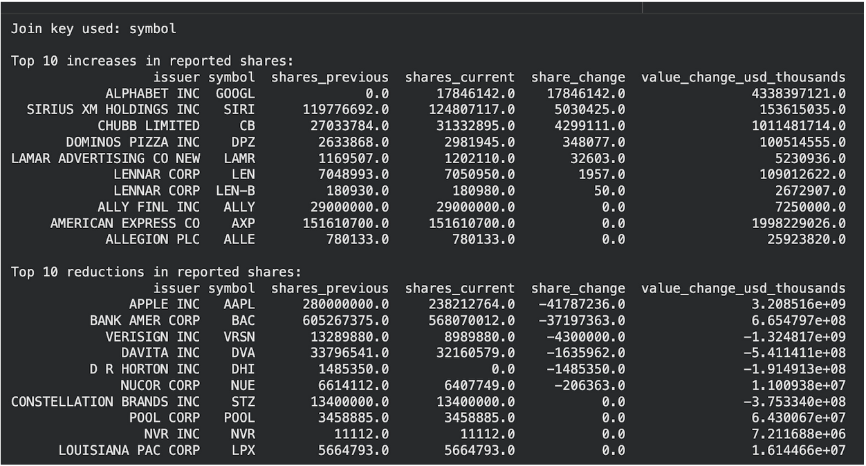
Interpretation of The Quarter-Over-Quarter Changes

The output compares two consecutive Form 13F filings for the same manager and tracks changes in reported share counts at the security level. Because share counts are used, the comparison reflects reported position adjustments rather than market price movement.

The join key used for alignment is the trading symbol, indicating that CUSIP identifiers were not consistently available across both filings for this comparison.

The top increases table highlights securities where reported share counts rose between quarters. Some entries represent newly disclosed positions, where the prior quarter shows zero shares. Others reflect incremental increases in existing holdings.

The top reductions table highlights securities where reported share counts declined. Negative values indicate partial reductions, while cases where current shares drop to zero represent reported exits from the disclosed long position.

The value change column reflects the change in reported position value associated with the share adjustment, expressed in thousands of dollars. This figure combines share changes and quarter-end pricing effects.

Overall, this output identifies where reported exposure increased, decreased, or exited between filing periods. It describes changes in disclosed holdings only and does not capture intraperiod trading, hedging activity, or net economic exposure.

Using 13F filings As an Institutional Signal Layer

Form 13F data works best when it strengthens a broader research stack instead of trying to act like a portfolio replica. The filing gives a consistent snapshot of reported long holdings at quarter end, which makes it useful for pattern recognition across managers and across time.

The concentration output functions as a structural indicator. A concentrated filing shows that a small set of positions dominates disclosed exposure. When you track this across multiple quarters, changes in top-holding weights and concentration metrics show whether the disclosed long book is becoming more focused or more distributed.

The quarter-over-quarter output functions as a change indicator. It surfaces which positions were initiated, increased, reduced, or exited at reporting dates. When you repeat the same comparison over several quarters, you can separate persistence from noise and avoid overreacting to a single filing.

At the signal-layer level, the goal is not to replicate positions. The goal is to identify where institutional exposure is consistently clustering and where reported allocations are shifting. These signals become more meaningful when combined with market context, such as price performance during the reporting window, earnings events, and fundamental changes. A practical way to structure that stack is outlined in FMP's overview of smart money tracking with 13F APIs, which connects filings discovery, holdings extraction, and monitoring.

A disciplined approach treats 13F-derived metrics as descriptive inputs. They help frame institutional behavior, but they do not capture hedging, shorts, derivatives, or intraperiod trading. For that reason, 13F signals should inform research workflows and monitoring, not act as standalone trade triggers.

Conclusion

Form 13F filings offer structured visibility into reported long equity holdings, but their value depends on how they are used. Read in isolation, they describe positions at a single point in time. Read systematically, they become a reliable signal layer.

By converting filings into datasets, measuring concentration, and tracking multi-quarter share changes, the data begins to show patterns rather than snapshots. These patterns highlight persistence, crowding, and directional shifts in disclosed exposure without assuming intent or strategy.

The key is restraint. 13F data supports analysis; it does not replace it. When combined with prices, earnings, and fundamentals, it adds institutional context. When overinterpreted, it misleads. Used with discipline, it strengthens long-term, evidence-based research.