Analyst Estimate Ranges by Sector and Fiscal Horizon: A Reproducible Methodology

An FMP Signals Lab Research Methodology

Version 1.0. Effective October 2026.

What Forecast Disagreement Measures

Most analysis of analyst estimates uses one number: the consensus. A company is expected to earn some amount next year, the stock trades against that expectation, and the figure that gets quoted is the average of whatever the covering analysts submitted.

The average is a summary of a distribution, and a summary discards information. Twelve analysts whose estimates sit close together produce the same consensus as twelve whose estimates are far apart. The average is identical. The spread around it is not.

This methodology measures that spread. Specifically, it measures the normalized high-low estimate range: the distance between the highest and lowest published estimate, divided by the size of the average. It describes how widely the published estimates are spread. It does not reveal the full distribution of individual forecasts, what any analyst knows, or how accurate the estimates will prove to be. A narrow range is consistent with agreement, and it is equally consistent with few contributors or with analysts anchored to the same guidance.

The measure is also only readable against something. The same range sits in very different positions depending on the company's industry, because businesses are forecast under different conditions. A utility's earnings follow an approved rate base closely; a refiner's move with margins that are difficult to forecast. A comparison across the two reflects the industries as much as the estimates.

This methodology therefore computes the normalized range from disclosed estimate data, places each company within the distribution of its sector, and reports the range across the available fiscal periods. It is descriptive. It reports what the estimate ranges look like and where a company sits among comparable companies. It does not score companies, rank sectors, or suggest what any of it implies for a security's price.

The Limits of Consensus-Only Analysis

The Consensus Is a Summary, and Summaries Hide Their Inputs

The consensus estimate is the most widely used number in equity research and one of the least informative on its own. It reports the centre of a distribution while discarding its width.

Two companies can carry the same consensus under different conditions. In one, the published estimates sit close together. In the other, they are far apart and the average sits between very different views. An analysis that reads only the consensus treats these as the same situation.

The problem is not that the consensus is wrong. It answers a narrower question than most readers assume.

Raw Spreads Are Not Comparable Across Sectors

The obvious response is to look at the range as well as the average. But a raw range compared across companies in different industries reflects the industry as much as the estimates.

Some businesses are forecast against relatively stable drivers, such as a regulated return or a contracted revenue base. Others are forecast against inputs that move unpredictably, such as commodity prices or product cycles. Estimate ranges tend to be wider in the second group, whatever the reason in any individual case.

An unadjusted comparison therefore largely reproduces the sector structure, a ranking of industries wearing the costume of a signal. Placing each company within its sector's distribution is what allows a range to be read against comparable companies.

A Large Range Is Not Automatically a Small Denominator

When the denominator of a ratio approaches zero, the ratio grows without limit, so a company forecast to earn almost nothing can show an enormous normalized range for arithmetic reasons.

In this data the concern applies narrowly rather than generally. Grouping companies by the size of their average earnings estimate at the primary horizon, the median normalized range is 0.082 for averages between fifty cents and a dollar (seven companies), 0.130 between one and two dollars (24), 0.115 between two and five dollars (111), 0.106 between five and ten dollars (139), and 0.100 above ten dollars (216). Across that span there is no systematic tendency for smaller averages to produce larger ranges. Only two companies have averages below fifty cents, too few to summarise.

The exception is the company forecast to break even, whose average sits within a few cents of zero and whose ratio is produced almost entirely by the denominator. Those cases are flagged individually and kept out of group statistics. They are not a reason to cap or discard large ratios in general, which would also remove observations reflecting wide published ranges on ordinary estimates.

Coverage Depth Has to Be Assessed, Not Assumed

A range measured across many estimates has more opportunity to be wide than one measured across a few, so the normalized range may partly reflect how many analysts contribute.

In this universe it does. Among the 493 companies with a valid earnings observation entering group statistics at the primary horizon, the Spearman rank correlation between the number of contributing analysts and the normalized range is 0.252. That is a positive but modest relationship: companies with more contributors tend to show wider ranges.

The relationship is not uniform. Within sectors it runs from 0.274 in Healthcare, 0.246 in Technology and 0.234 in Industrials to negative values in Utilities, Communication Services and Basic Materials. Several sectors contain between seventeen and thirty-two companies, so their individual coefficients are imprecise and should not be read as stable sector characteristics.

The framework does not adjust for coverage, because an adjustment would be a further modelling choice with assumptions of its own. It reports the number of contributing analysts on every observation instead, and treats coverage as a factor a reader has to weigh. A wide range across many analysts and a wide range across a few are not the same observation.

The Data Behind Forecast Disagreement

What Arrives as Structured Fields

For each company and each fiscal period, the estimates endpoint returns the low, high, and average projection for revenue, EBITDA, EBIT, net income, and earnings per share, together with separate counts of the analysts contributing to the revenue and earnings figures. Sector and sub-sector labels arrive from the index constituent endpoint alongside the company list, so the universe and its classification come from a single call.

There is no document to parse. The work is universe construction, validation of every estimate range, and arithmetic.

Coverage and Validity for a Dated Run

For the snapshot reported on this page, retrieved on 29 September 2026, the index returned 503 listings representing 500 companies once multiple share classes were resolved. Every company returned estimate data. One, Loews, had no fiscal period falling at the primary horizon described below, leaving 499 earnings observations.

All 499 passed the validity checks set out in the engineering section, and some carry flags: three ranges crossing zero, three observations with fewer than three contributing analysts, one average close to zero, and two negative averages. A range crossing zero, a near-zero average, or low coverage keeps an observation in company-level output but makes it ineligible for group statistics; a negative average alone does not. That leaves 493 companies eligible for the sector distributions for earnings. For revenue the figure is 495, with four observations flagged for low coverage.

These counts belong to this snapshot. A later run queries estimates as they stand on its own date and will produce different counts, and each study reports its own.

The Time Dimension Is Fiscal, Not Calendar

Estimates are keyed to the fiscal period they describe, not to the date on which they were made. A request returns projections for several periods forward and several back, but nothing indicates when any of them was formed or last revised. A cross-section can be measured completely today; the previous cross-section cannot be recovered unless it was stored at the time.

Fiscal calendars also differ. One company's fiscal year ends in December, another's in September, another's in January. Grouping periods by the calendar year in which they end would label a period four months away and one sixteen months away as the same horizon.

The framework instead indexes each company's own periods from the date of observation. The first period ending on or after that date, compared as calendar dates, is the fiscal year in progress, labelled H0; a period ending on the observation date itself counts as H0. The year after it is H+1, the primary horizon for comparisons on this page. Every observation carries its actual period-end date and the months remaining to it. At the primary horizon those months fall between roughly twelve and twenty-four, depending on the fiscal calendar, and the difference is reported rather than removed.

Annual Periods Only

The estimates endpoint returns both annual and quarterly periods. This methodology uses the annual series only. Its measures, sector comparisons and horizons are all defined at the fiscal-year level, and extending the framework to quarterly periods would require its own validation of horizons and coverage. That extension is outside its scope.

Two Structural Adjustments

A small number of companies list more than one share class. Their estimates are close but not identical, and the number of contributing analysts differs, so counting both would weight one company twice in its sector. The framework identifies these by central index key and keeps one listing, chosen by the rule set out in the engineering section.

A company whose average estimate sits within a few cents of zero produces a ratio that is arithmetically valid and dominated by its denominator. That case, and several others, are handled by explicit validity rules rather than by a general cap.

Why Standard Approaches Miss the Signal

An analyst who moves past the consensus to the estimate range can still reach the wrong conclusion, because the range carries traps of its own. Four recur.

Ranking Companies Across Sectors

The most common error is also the easiest to make. Having computed ranges for a universe, the natural next step is to sort them, and the resulting list looks like a signal.

It is mostly a list of industries. The companies at the top will be concentrated in a handful of sectors where estimate ranges are typically wide, and those at the bottom in sectors where they are typically narrow. Sorting the universe by raw range therefore largely reproduces the sector structure. Whether a company's range is unusual among comparable companies is invisible until it is placed within its sector.

Assuming a Large Ratio Means a Small Denominator

The second trap is the correction to the first, applied too broadly. Ratios misbehave when their denominator approaches zero, and the instinct is to treat every large figure as suspect and cap or exclude it.

In this data that instinct removes observations worth keeping. Several of the widest ranges come from ordinary average estimates and published ranges of several dollars per share. Capping them would discard those along with the genuine break-even cases.

The narrow version of the concern is real and is handled case by case. The general version, applied as a blanket rule, does more damage than the problem it addresses.

Comparing Fiscal Years as If They Were Calendar Years

The third trap is quieter. Estimate periods arrive labelled with their end dates, and the natural shortcut is to group them by year: everything ending in 2027 is next year's estimate.

It is not. A company whose fiscal year ends in January 2027 is, in September 2026, partway through that year. A company whose fiscal year ends in December 2027 has not started it. Grouping the two by calendar year places a year in progress alongside one more than a year away, and ranges at different distances from their period end are not directly comparable.

The framework indexes each company's periods from the observation date instead, and reports the months remaining to each period end, so differences in fiscal calendar are visible rather than absorbed into the comparison.

Ignoring How Many People Contributed

The final trap is reading a range without knowing how many estimates produced it. A range across four analysts and a range across forty are different kinds of evidence, even when the number is the same.

In this universe the difference is not only conceptual. Companies with more contributing analysts tend to show wider ranges, and both the strength and the direction of that relationship vary by sector. Coverage is therefore something a reader has to weigh for each observation, and the framework reports it on every one.

These four are independent. Placing a company within its sector does nothing about a break-even denominator, and neither addresses a mismatch in fiscal calendars. The framework that follows handles each explicitly.

What Has to Be Engineered

The previous section described the analytical traps. This section sets out the rules that avoid them across a full index. The inputs arrive as structured numbers, so the work is smaller than in a filings-based methodology, but each rule below is stated so that a reader reproducing the results makes the same decisions.

Constructing the Universe

The universe is the S&P 500 as returned by the index constituent endpoint, which supplies each company's symbol, sector, sub-sector and central index key in a single call. A listing with no sector or no central index key is excluded with a logged reason. A missing sub-sector is recorded as Unclassified.

Companies listing more than one share class appear once per class. Their estimates are close but not identical, because different analysts cover each line. The framework groups listings by central index key and keeps one per company: the listing with more analysts contributing to the earnings estimate at the primary horizon, and where those counts are equal, the alphabetically first symbol. The tie-breaker exists so that the same inputs always produce the same universe.

Defining the Horizon

Each company's fiscal periods are indexed from the date of observation rather than grouped by calendar year. The first period ending on or after the observation date, comparing calendar dates rather than timestamps, is H0, the fiscal year in progress. Every other period is placed by the number of whole fiscal years between it and H0: the year after is H+1, the primary horizon for sector comparisons, and completed years run H-1 backward.

Counting years rather than rows matters when the data is incomplete. If a fiscal year is missing, the next available year keeps its true position, H+2 rather than H+1, and the gap is logged instead of closing silently. A period date that cannot be read is logged. Two rows for the same period date are kept once if they are identical and excluded if they conflict, and either case is logged. A period that does not fall within 0.15 years of a whole number of years from H0, as happens when a company changes its fiscal year end, is logged and excluded, because its horizon cannot be assigned reliably.

Every observation carries its actual period-end date and the number of months remaining to it. Because fiscal years end in different months, the months remaining at H+1 range from roughly twelve to twenty-four across companies. The framework reports that difference rather than adjusting for it.

Choosing the Series

The framework uses annual periods only. Its measures, comparisons and horizons are defined at the fiscal-year level, and applying them to quarterly periods would require separate validation. That is a scope decision, stated so that a reader knows which series every figure comes from.

Validity Rules

Every estimate range is assessed before it is used. The rules apply separately to earnings per share and to revenue, each with its own analyst count.

An observation is invalid, and excluded with a logged reason, if a low, high or average value is missing; if any value is not a finite number; if the high is below the low; if the average falls outside the reported range; or if the average is exactly zero. These rules apply at every horizon, and every invalid observation is written to the exclusions log with its horizon.

A valid observation is flagged, and kept in company-level output but made ineligible for group statistics, in four cases: its absolute average is below a near-zero threshold of $0.05 per share for earnings or $1,000,000 for revenue; its range crosses zero, with the low below zero and the high above it; its analyst count is missing, or is not a finite, nonnegative whole number; or fewer than three analysts contributed to that metric.

Two of these are choices this framework makes rather than mathematical necessities. When a range crosses zero, the ratio is still defined as long as the average is not zero, but the published estimates disagree about whether the result will be a profit or a loss, and the framework excludes such observations from group comparisons rather than placing them on the same scale as the rest. Likewise, any two estimates form a range; three contributing analysts is the minimum this framework sets before an observation contributes to a group statistic.

A negative average whose range does not cross zero is flagged and remains eligible for group statistics, because the ratio is well defined against the absolute value of the average. The flag records the fact without excluding the observation.

Normalizing Without Flattening

A company's normalized range is read against the distribution of its sector at the same horizon. Group statistics use only observations eligible for group statistics: valid observations carrying none of the excluding flags above. Quartiles are computed with Python's statistics.quantiles using the inclusive method. Every sector and sub-sector present in the universe is reported with its count of eligible observations, including a count of zero; one with fewer than five reports that count and no median or quartiles.

The framework reports the company's range, the sector median, and the sector's quartiles together rather than a single normalized score. A company above a tightly clustered sector's median is a different observation from one the same distance above a widely dispersed sector's median.

Placing a company within its sector provides context. It does not remove every source of difference. Companies in the same sector still differ in business mix, analyst coverage and months remaining to period end, and a sector median absorbs none of those.

Storing What Cannot Be Recovered

Because estimates carry no observation date, a cross-section cannot be reconstructed after the moment has passed. The framework therefore stores every run.

Each run writes to a directory named for its UTC timestamp: the raw constituent and estimate responses, a manifest recording the methodology version, observation time, endpoints, every parameter, the focus sector and the term-structure company, a log of every exclusion and request failure, and the computed outputs.

A live run always creates a new snapshot of estimates as they stand that day, so it will not reproduce figures published from an earlier date. Reproducing a published figure requires the snapshot it came from. Setting the replay path to that snapshot reruns the calculation from its stored inputs without contacting the data source, and restores the settings recorded in its manifest rather than the script's current values. Replay stops if the snapshot's methodology version differs from the script's, and warns where a snapshot predates a field the script now records.

How FMP Supports the Workflow

Defining the Universe With the S&P 500 Index API

The S&P 500 Index API returns the index constituents with their symbol, company name, sector, sub-sector, central index key, and headquarters. One call supplies both the universe and its classification, so every company in a run is labelled by the same source at the same moment. The central index key in the same response is what makes the share-class rule possible without relying on ticker conventions.

Reading Estimate Ranges With the Financial Estimates API

The Financial Estimates API supplies the measurements. For each company and fiscal period it returns low, high, and average projections for revenue, EBITDA, EBIT, net income, and earnings per share, with separate counts of the analysts contributing to the revenue and earnings figures.

The low and high are the fields this methodology is built on, and they are the fields consensus-focused analysis usually discards. Their presence as returned values is what makes the normalized range computable across a full index.

The endpoint accepts an annual or quarterly period and a limit, which is how the framework selects its series and the number of periods retrieved.

Checking Sector Labels With Company Profiles

The Company Profile Data API returns sector and industry for an individual company. The reference script does not call it. Every classification in this run comes from the S&P 500 constituent list, so that each company is labelled by the same source at the same moment. The profile endpoint is an optional independent check on that classification, and a route for extending the method to companies outside the index, where no constituent list supplies a sector.

Dividing Responsibilities Between FMP and the Methodology

FMP supplies the universe, the classification, and the estimate ranges as structured values. The methodology supplies the universe rules, the horizon definition, the validity rules, the sector comparison, and the storage that makes any figure reproducible.

Framework Design

The framework starts from the disclosed estimate range and derives five measures from it. There is no composite score. Each measure is reported separately with the context needed to read it, because combining them would require weights this methodology does not attempt to justify.

1. The Base Unit

The base unit is the set of disclosed fields for one company, one metric, and one fiscal period: the low, the high, and the average projection, the number of contributing analysts for that metric, the period-end date, and the months remaining to it. These are facts rather than measures, and every measure below is derived from them.

2. Dispersion

Dispersion is the normalized high-low estimate range: the high estimate minus the low, divided by the absolute value of the average. It expresses the width of the published range in proportion to the size of the estimate, which is what makes it comparable between a company expected to earn two dollars and one expected to earn twenty.

It is always reported with the absolute range in currency terms and the validity flags. The two figures together distinguish a wide range on an ordinary estimate from a narrow range on an estimate close to zero, which can produce similar ratios and mean entirely different things.

It is computed on earnings per share as the primary metric and on revenue as a secondary one, each with its own analyst count. The two frequently disagree, and the disagreement is informative in its own right.

3. Sector Position

Sector position places a company's normalized range against the median and quartiles of its sector at the same horizon, using observations eligible for group statistics.

Raw ranges are not comparable across sectors, so the comparison is made within them. The result is reported as the company's range alongside the sector's median and quartiles, not as a single normalized figure. It provides context rather than a controlled comparison: differences in coverage, business mix and months to period end remain within any sector.

4. Term Structure

Term structure is the normalized range for the same company across its fiscal periods, as observed in a single retrieval, from completed years through the furthest forward estimate available.

It shows how ranges differ at one moment between periods already completed and periods still ahead. It does not show that the range for any individual period narrowed or widened over time. That can only be established by comparing stored snapshots, and the framework makes no claim about change until such snapshots exist.

5. Sub-Sector Composition

Sub-sector composition breaks a sector down by the sub-sector labels attached to its constituents. Every sub-sector in the sector is reported with its count of eligible observations, even when that count is zero. Sub-sectors reaching the five-observation minimum report a median and quartiles; smaller ones report none, and list their companies individually, each with any flags it carries.

In large sectors this produces meaningful group comparisons. In small ones, most sub-sectors fall below the minimum, and the composition is read through individual values rather than group statistics.

6. Coverage Depth

Coverage depth is the number of analysts contributing to each metric, reported alongside every observation.

It is context rather than a scored signal. In this universe it is positively related to the normalized range, modestly and unevenly across sectors, so it is a factor a reader has to weigh when interpreting any single observation. The framework reports it rather than adjusting for it.

What the Framework Produces

Each run produces a set of stored files. An observations table carries every company, metric and period with its low, high and average, absolute and normalized range, analyst count, period-end date, months remaining, validity status and flags. A sector positions table places each company against its sector at the primary horizon. Sector profiles give the count, median and quartiles for both metrics. An exclusions log records every listing, period or observation removed and why, at every horizon. A diagnostics file carries the coverage and denominator statistics, and a manifest records how the run was produced, including every setting needed to replay it.

There is no combined score and no ranking. Comparisons are made measure by measure, and across sectors only through sector distributions.

Reproducing the Measures With FMP

This walkthrough runs the framework across the S&P 500. Each stage states the decision it implements, gives the code, shows the output, and interprets the result.

The figures below come from the snapshot retrieved on 29 September 2026, processed by replaying it with the reference implementation in the next section. That snapshot was taken before the script recorded its focus sector, term-structure company and spacing tolerance, and before the two analyst-count flags were added, so Stage 1 opens with four warnings to that effect. None changes a figure: no observation in the snapshot has a missing or invalid analyst count or a period-date issue, and the sector and company selected by rule are the ones shown.

Before You Run This Code

You will need Python 3.9 or later and the requests library. A live run also needs an FMP API key in the API_KEY variable; it creates a new timestamped directory under snapshots and describes the estimates as they stand that day. Replaying a stored snapshot needs no key: set REPLAY_DIR to its directory. The full script appears in the next section.

Stage 1: Build the Universe

Purpose. The S&P 500 Index API supplies the constituents with their sector, sub-sector, and central index key. Listings are grouped by that key and reduced to one per company before anything is measured.

def build_universe(src): rows = src.get("constituents.json", "sp500-constituent", {}) or [] excluded, by_cik = [], defaultdict(list) for c in rows: sym = c.get("symbol") if not sym: excluded.append(("?", "universe", "missing_symbol")); continue if not c.get("sector"): excluded.append((sym, "universe", "missing_sector")); continue if not c.get("cik"): excluded.append((sym, "universe", "missing_cik")); continue by_cik[str(c["cik"])].append(c) return rows, by_cik, excluded def resolve_share_classes(by_cik, coverage): """One listing per company. Keep the class with more contributing EPS analysts; if equal, keep the alphabetically first symbol.""" universe, collapsed = {}, [] for cik, listings in by_cik.items(): if len(listings) == 1: universe[listings[0]["symbol"]] = listings[0] continue ranked = sorted(listings, key=lambda c: (-(coverage.get(c["symbol"]) or 0), c["symbol"])) keep = ranked[0] universe[keep["symbol"]] = keep collapsed.append((cik, [c["symbol"] for c in listings], keep["symbol"])) return universe, collapsed

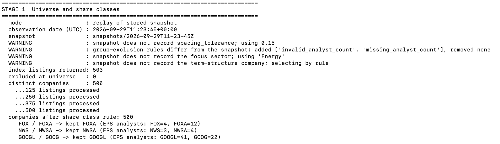
Stage 1 output - universe and share classes

Interpretation. 503 listings resolve to 500 companies. All three collapsed pairs sit in Communication Services, and in each case the retained listing has more contributing analysts: Alphabet's Class A with 41 against 22 for Class C, and the corresponding choice at Fox and News Corporation.

The adjustment is small in count and not in effect. Without it, Communication Services would count twenty-two listings for nineteen companies, measuring Alphabet twice and shifting the median every other company in the sector is read against.

Stage 2: Assign Horizons and Assess Each Observation

Purpose. Each company's periods are indexed from the observation date, and every estimate range is checked against the validity rules before it enters any calculation.

def analyst_count(x): """A usable analyst count is a finite, nonnegative whole number.""" if x is None or x == "": return None, "missing_analyst_count" v = to_number(x) if v is None or not math.isfinite(v) or v < 0 or v != int(v): return None, "invalid_analyst_count" return int(v), None def assign_horizons(rows, observed_date): """Index a company's fiscal periods by whole years from the fiscal year in progress. H0 is the first period ending on or after the observation date, compared as calendar dates. Returns the periods and a list of issues; nothing is dropped without being recorded.""" issues, by_date = [], defaultdict(list) for r in rows: d = parse_date(r.get("date")) if d is None: issues.append("invalid_date") else: by_date[d].append(r) periods = [] for d in sorted(by_date): group = by_date[d] if len(group) > 1: if all(g == group[0] for g in group): issues.append("duplicate_period_identical:%s" % d.isoformat()) else: issues.append("duplicate_period_conflicting:%s" % d.isoformat()) continue periods.append((d, group[0])) if not periods: return [], issues future = [d for d, _ in periods if d >= observed_date] if future: anchor = future[0] else: anchor = periods[-1][0] while anchor < observed_date: day = 28 if (anchor.month, anchor.day) == (2, 29) else anchor.day anchor = anchor.replace(year=anchor.year + 1, day=day) out, seen = [], {} for d, r in periods: years = (d - anchor).days / 365.25 h = round(years) if abs(years - h) > SPACING_TOLERANCE: issues.append("irregular_period_spacing:%s" % d.isoformat()); continue if h in seen: issues.append("horizon_conflict:H%+d" % h); continue seen[h] = d out.append({"horizon": h, "period_end": d.isoformat(), "months_to_end": round((d - observed_date).days / 30.4375, 1), "row": r}) hs = sorted(seen) for h in range(hs[0], hs[-1] + 1): if h not in seen: issues.append("missing_annual_period:H%+d" % h) return out, issues def assess(metric, low, high, avg, analysts): """Status and flags for one estimate range.""" low, high, avg = to_number(low), to_number(high), to_number(avg) n, count_issue = analyst_count(analysts) base = {"low": low, "high": high, "avg": avg, "analysts": n, "spread": None, "ratio": None, "flags": [], "in_groups": False} if low is None or high is None or avg is None: return dict(base, status="invalid", reason="missing_field") if not all(math.isfinite(v) for v in (low, high, avg)): return dict(base, status="invalid", reason="non_finite") if high < low: return dict(base, status="invalid", reason="reversed_bounds") tol = 1e-9 * max(1.0, abs(high), abs(low)) if avg < low - tol or avg > high + tol: return dict(base, status="invalid", reason="average_outside_range") if avg == 0: return dict(base, status="invalid", reason="zero_average") spread = high - low flags = [] if abs(avg) < NEAR_ZERO[metric]: flags.append("near_zero") if low < 0 < high: flags.append("crosses_zero") if avg < 0: flags.append("negative_average") if count_issue: flags.append(count_issue) elif n < MIN_ANALYSTS: flags.append("low_coverage") return dict(base, status="valid", reason="", spread=spread, ratio=spread / abs(avg), flags=flags, in_groups=not (set(flags) & EXCLUDE_FROM_GROUPS))

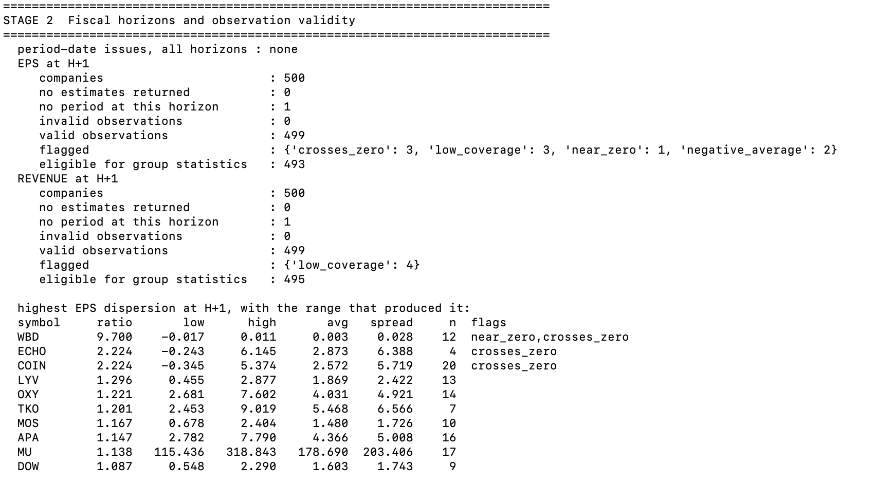
Stage 2 output - validity summary and widest ranges

Interpretation. No period date in the snapshot is missing, duplicated, unreadable or irregularly spaced. Of 500 companies, one has no fiscal period at the primary horizon, leaving 499 earnings observations. None is invalid at the primary horizon. Six carry flags that make them ineligible for group statistics, leaving 493. Across the other horizons, 24 earnings observations have an average of exactly zero and are excluded with a logged reason; 19 of them fall at the two most distant horizons.

The top of the table shows why the ratio is never reported alone. The widest normalized range in the universe belongs to a company with an average earnings estimate of three tenths of a cent and published estimates running from a loss of 1.7 cents to a profit of 1.1 cents. The range is under three cents; the ratio is 9.700 because the denominator is almost zero. It is flagged twice, as a near-zero average and as a range crossing zero.

Four rows below, a company with an average estimate of $4.03 shows a range from $2.68 to $7.60 across fourteen analysts. Its ratio is 1.221 and it carries no flags. Read as ratios alone, the first looks eight times as dispersed as the second. Read with the range beside them, the first is produced by its denominator and the second is a wide set of published estimates.

The second and third rows show a different case. Each has an ordinary average estimate, but at least one analyst forecasts a loss while others forecast a profit. Their ratios are well defined, since neither average is zero, but the framework excludes ranges that cross zero from group comparisons as a methodological choice. Both are flagged and kept out of group statistics while remaining in company-level output.

Stage 3: Place Companies Within Their Sector

Purpose. Ranges are not comparable across sectors. This stage computes each sector's median and quartiles from observations eligible for group statistics, for both earnings and revenue.

def quartiles(values): q = statistics.quantiles(values, n=4, method=QUARTILE_METHOD) return q[0], statistics.median(values), q[2] def group_profile(obs, key, metric, horizon, groups=()): """Statistics per group from observations eligible for group statistics. Every group named in `groups` is reported, including those with none.""" eligible = defaultdict(list) for o in obs: if (o["metric"] == metric and o["horizon"] == horizon and o["status"] == "valid" and o["in_groups"]): eligible[o[key]].append(o["ratio"]) profile = {} for g in set(groups) | set(eligible): v = eligible.get(g, []) if len(v) < MIN_GROUP: profile[g] = {"n": len(v), "reported": False} continue p25, med, p75 = quartiles(v) profile[g] = {"n": len(v), "reported": True, "p25": p25, "median": med, "p75": p75} return profile

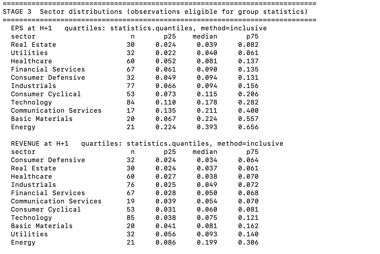
Stage 3 output - sector distributions for earnings and revenue

Interpretation. For earnings, sector medians run from 0.039 in Real Estate to 0.393 in Energy, roughly a tenfold range. A company with a normalized range of 0.18 sits well above the median in Real Estate, well below it in Energy, and close to it in Technology at 0.178. The same figure occupies three different positions depending on the sector.

The quartiles matter as much as the medians. Utilities is tightly clustered, with its middle half between 0.022 and 0.061. Basic Materials has a median of 0.224 and an upper quartile of 0.557, a compact majority with a long upper tail. Two companies equally far above their sector medians are not equally unusual.

The revenue table shows why the framework carries both metrics. Utilities has the second-narrowest earnings range at 0.040 and the second-widest revenue range at 0.093. That pattern is consistent with regulated earnings alongside revenue that passes fuel costs through to customers, though the data shows the divergence rather than its cause. Reading either metric alone would give a different picture of the same sector.

Stage 4: Read the Term Structure

Purpose. This stage reads the normalized range for one company across its fiscal periods, as observed in a single retrieval.

def term_structure(obs, symbol, metric="eps"): rows = [o for o in obs if o["symbol"] == symbol and o["metric"] == metric] return sorted(rows, key=lambda o: o["horizon"])

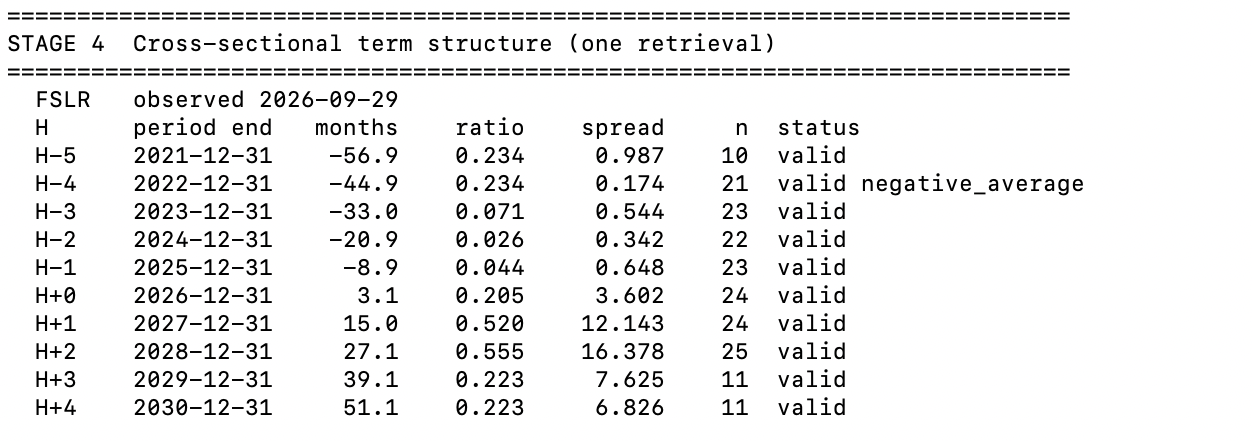
Stage 4 output - one company across fiscal periods

Interpretation. At the moment of retrieval, the range for the company's completed years is low: 0.026 for the year ended December 2024. For periods still ahead it is higher: 0.205 for the year in progress, three months from its end, 0.520 for the next year and 0.555 for the one after. The absolute range moves further still, from 34 cents to over sixteen dollars.

This is a pattern across periods observed at one moment. It does not show that the range for any particular period narrowed as that period approached; only snapshots compared over time can show that.

The two most distant periods show a lower ratio of 0.223, but the number of contributing analysts falls there from around 25 to 11. Given the positive relationship between coverage and range, the lower figure may partly reflect fewer contributors rather than a narrower set of views.

Stage 5: Break a Sector Down by Sub-Sector

Purpose. A sector median describes a group that is rarely uniform. This stage splits one sector by sub-sector, reporting every sub-sector with its count of eligible observations, and a median only where the five-observation minimum is met.

def sub_sector_split(obs, universe, sector, metric="eps", horizon=None): """Every sub-sector in the sector is reported, with its count of eligible observations. Valid observations are listed with their flags, whether or not they enter the group statistic.""" horizon = PRIMARY_HORIZON if horizon is None else horizon subs = {c.get("subSector") or "Unclassified" for c in universe.values() if c["sector"] == sector} scoped = [o for o in obs if o["sector"] == sector] profile = group_profile(scoped, "sub_sector", metric, horizon, groups=subs) members = defaultdict(list) for o in scoped: if (o["metric"] == metric and o["horizon"] == horizon and o["status"] == "valid"): members[o["sub_sector"]].append(o) return profile, members

Stage 5 output - Energy by sub-sector

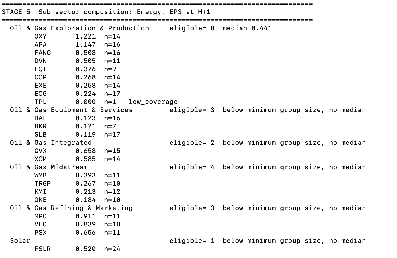
Interpretation. Only one Energy sub-sector reaches the minimum: exploration and production, with a median of 0.441 across eight eligible companies. The others contain between one and four companies each, so the framework lists their members individually and computes no median for them.

The individual values still show how uneven the sector is. The three refiners sit at 0.911, 0.839 and 0.656; the three equipment and services companies at 0.123, 0.121 and 0.119. That is a difference of roughly five to eight times between two groups under the same sector heading, though neither group is large enough to support a group statistic.

A ninth exploration and production company shows a range of exactly zero, with a single contributing analyst. One estimate cannot form a range, so the zero reflects coverage rather than agreement. It is flagged and excluded from the sub-sector median.

In smaller sectors like this one, sub-sector composition is read mostly through individual values. It carries more analytical weight in large sectors, where more sub-sectors reach the minimum size.

Complete Reference Implementation

The staged walkthrough explains each decision separately. The script below combines them into one workflow. With an FMP API key and REPLAY_DIR left as None, it runs live: it queries the API, writes a new snapshot, and reports estimates as they stand that day, which will differ from the figures on this page. With REPLAY_DIR set to a stored snapshot, it reads that snapshot's inputs and settings instead and calls nothing. The figures on this page come from a stored run of 29 September 2026, so a reader's own live run will produce different figures, reflecting the estimates on the day it runs. Keeping each run's snapshot is what allows that run to be reproduced exactly later.

""" Estimate Dispersion: reference implementation, version 1.0. Stage 1 Build the universe and resolve multi-class listings. Stage 2 Assign fiscal horizons and assess every observation. Stage 3 Compute sector distributions from eligible observations. Stage 4 Read the cross-sectional term structure for one company. Stage 5 Break a sector down by sub-sector. A live run queries the API and stores its raw inputs, settings and outputs in a new timestamped snapshot. Because estimates change continuously, a live run describes the day it is taken and will not reproduce earlier figures. To reproduce a published run, set REPLAY_DIR to its snapshot: replay reads the stored inputs and restores the stored settings, without calling the API. """ import requests, statistics, json, csv, math, os, time from collections import defaultdict from datetime import datetime, timezone # ---------------------------------------------------------------- settings API_KEY = "YOUR_FMP_API_KEY" BASE = "https://financialmodelingprep.com/stable" METHODOLOGY_VERSION = "1.0" SNAPSHOT_ROOT = "snapshots" REPLAY_DIR = None # e.g. "snapshots/2026-09-29T11-23-45Z" FOCUS_SECTOR = "Energy" # sector broken down in Stage 5 TERM_SYMBOL = None # Stage 4 company; None picks the most-covered in FOCUS_SECTOR PRIMARY_HORIZON = 1 # next fiscal year after the one in progress ESTIMATE_LIMIT = 10 # annual periods requested per company NEAR_ZERO = {"eps": 0.05, # dollars per share "revenue": 1_000_000.0} # dollars MIN_ANALYSTS = 3 # this framework's minimum contributors for a group statistic MIN_GROUP = 5 # minimum eligible observations for a group statistic QUARTILE_METHOD = "inclusive" # statistics.quantiles convention SPACING_TOLERANCE = 0.15 # years off a whole-year step before a period counts as irregular # flags that keep an observation at company level but out of group statistics EXCLUDE_FROM_GROUPS = {"near_zero", "crosses_zero", "low_coverage", "missing_analyst_count", "invalid_analyst_count"} METRICS = { "eps": ("epsLow", "epsHigh", "epsAvg", "numAnalystsEps"), "revenue": ("revenueLow", "revenueHigh", "revenueAvg", "numAnalystsRevenue"), } TUNABLE = ["primary_horizon", "limit", "near_zero", "min_analysts", "min_group", "quartile_method", "spacing_tolerance"] def current_settings(): return {"primary_horizon": PRIMARY_HORIZON, "limit": ESTIMATE_LIMIT, "near_zero": NEAR_ZERO, "min_analysts": MIN_ANALYSTS, "min_group": MIN_GROUP, "quartile_method": QUARTILE_METHOD, "spacing_tolerance": SPACING_TOLERANCE} def apply_settings(params): """Restore the settings a snapshot was produced with.""" global PRIMARY_HORIZON, ESTIMATE_LIMIT, NEAR_ZERO, MIN_ANALYSTS global MIN_GROUP, QUARTILE_METHOD, SPACING_TOLERANCE PRIMARY_HORIZON = params["primary_horizon"] ESTIMATE_LIMIT = params["limit"] NEAR_ZERO = {k: float(v) for k, v in params["near_zero"].items()} MIN_ANALYSTS = params["min_analysts"] MIN_GROUP = params["min_group"] QUARTILE_METHOD = params["quartile_method"] SPACING_TOLERANCE = params["spacing_tolerance"] # ---------------------------------------------------------------- source class Source: """Fetches from the API and saves every raw response, or replays a saved snapshot. Failures are recorded, never silently skipped.""" def __init__(self, replay_dir=None): self.replay = replay_dir self.failures = [] if replay_dir: self.root = replay_dir with open(os.path.join(replay_dir, "manifest.json")) as f: self.manifest = json.load(f) else: stamp = datetime.now(timezone.utc).strftime("%Y-%m-%dT%H-%M-%SZ") self.root = os.path.join(SNAPSHOT_ROOT, stamp) os.makedirs(os.path.join(self.root, "raw", "estimates"), exist_ok=True) self.manifest = None def get(self, relpath, endpoint, params): path = os.path.join(self.root, "raw", relpath) if self.replay: if not os.path.exists(path): self.failures.append((relpath, "missing_from_snapshot")) return None with open(path) as f: return json.load(f) p = dict(params); p["apikey"] = API_KEY try: r = requests.get(BASE + "/" + endpoint, params=p, timeout=45) except requests.RequestException as e: self.failures.append((relpath, "request_error:" + type(e).__name__)) return None if r.status_code != 200: self.failures.append((relpath, "http_%d" % r.status_code)) return None try: data = r.json() except ValueError: self.failures.append((relpath, "invalid_json")) return None if not isinstance(data, list): self.failures.append((relpath, "unexpected_payload")) return None with open(path, "w") as f: json.dump(data, f) return data def restore_replay(src): """Check the snapshot's version and restore its settings. Stops on a version mismatch; warns where the snapshot predates a recorded field.""" global FOCUS_SECTOR, TERM_SYMBOL m = src.manifest if m.get("methodology_version") != METHODOLOGY_VERSION: raise SystemExit("Snapshot methodology version %r does not match this script (%r). " "Replay stopped." % (m.get("methodology_version"), METHODOLOGY_VERSION)) params = m.get("parameters", {}) restored, warnings = current_settings(), [] for k in TUNABLE: if k in params: restored[k] = params[k] else: warnings.append("snapshot does not record %s; using %r" % (k, restored[k])) apply_settings(restored) recorded = set(params.get("exclude_from_groups", [])) if recorded and recorded != EXCLUDE_FROM_GROUPS: warnings.append("group-exclusion rules differ from the snapshot: added %s, removed %s" % (sorted(EXCLUDE_FROM_GROUPS - recorded) or "none", sorted(recorded - EXCLUDE_FROM_GROUPS) or "none")) if "focus_sector" in m: FOCUS_SECTOR = m["focus_sector"] else: warnings.append("snapshot does not record the focus sector; using %r" % FOCUS_SECTOR) if "term_symbol" in m: TERM_SYMBOL = m["term_symbol"] else: warnings.append("snapshot does not record the term-structure company; selecting by rule") return warnings # ---------------------------------------------------------------- helpers def to_number(x): if x is None or x == "" or isinstance(x, bool): return None try: return float(x) except (TypeError, ValueError): return None def analyst_count(x): """A usable analyst count is a finite, nonnegative whole number.""" if x is None or x == "": return None, "missing_analyst_count" v = to_number(x) if v is None or not math.isfinite(v) or v < 0 or v != int(v): return None, "invalid_analyst_count" return int(v), None def parse_date(s): try: return datetime.strptime(str(s)[:10], "%Y-%m-%d").date() except (TypeError, ValueError): return None def quartiles(values): q = statistics.quantiles(values, n=4, method=QUARTILE_METHOD) return q[0], statistics.median(values), q[2] def ranks(values): order = sorted(range(len(values)), key=lambda i: values[i]) r = [0.0] * len(values) i = 0 while i < len(order): j = i while j + 1 < len(order) and values[order[j + 1]] == values[order[i]]: j += 1 avg = (i + j) / 2.0 + 1 for k in range(i, j + 1): r[order[k]] = avg i = j + 1 return r def spearman(x, y): if len(x) < 3: return None rx, ry = ranks(x), ranks(y) mx, my = statistics.mean(rx), statistics.mean(ry) num = sum((a - mx) * (b - my) for a, b in zip(rx, ry)) den = math.sqrt(sum((a - mx) ** 2 for a in rx) * sum((b - my) ** 2 for b in ry)) return num / den if den else None def show_count(n): return "%d" % n if isinstance(n, int) else "-" # ------------------------------------------------- Stage 1: the universe def build_universe(src): rows = src.get("constituents.json", "sp500-constituent", {}) or [] excluded, by_cik = [], defaultdict(list) for c in rows: sym = c.get("symbol") if not sym: excluded.append(("?", "universe", "missing_symbol")); continue if not c.get("sector"): excluded.append((sym, "universe", "missing_sector")); continue if not c.get("cik"): excluded.append((sym, "universe", "missing_cik")); continue by_cik[str(c["cik"])].append(c) return rows, by_cik, excluded def resolve_share_classes(by_cik, coverage): """One listing per company. Keep the class with more contributing EPS analysts; if equal, keep the alphabetically first symbol.""" universe, collapsed = {}, [] for cik, listings in by_cik.items(): if len(listings) == 1: universe[listings[0]["symbol"]] = listings[0] continue ranked = sorted(listings, key=lambda c: (-(coverage.get(c["symbol"]) or 0), c["symbol"])) keep = ranked[0] universe[keep["symbol"]] = keep collapsed.append((cik, [c["symbol"] for c in listings], keep["symbol"])) return universe, collapsed # ------------------------------------------------- Stage 2: horizons and validity def assign_horizons(rows, observed_date): """Index a company's fiscal periods by whole years from the fiscal year in progress. H0 is the first period ending on or after the observation date, compared as calendar dates. Returns the periods and a list of issues; nothing is dropped without being recorded.""" issues, by_date = [], defaultdict(list) for r in rows: d = parse_date(r.get("date")) if d is None: issues.append("invalid_date") else: by_date[d].append(r) periods = [] for d in sorted(by_date): group = by_date[d] if len(group) > 1: if all(g == group[0] for g in group): issues.append("duplicate_period_identical:%s" % d.isoformat()) else: issues.append("duplicate_period_conflicting:%s" % d.isoformat()) continue periods.append((d, group[0])) if not periods: return [], issues future = [d for d, _ in periods if d >= observed_date] if future: anchor = future[0] else: anchor = periods[-1][0] while anchor < observed_date: day = 28 if (anchor.month, anchor.day) == (2, 29) else anchor.day anchor = anchor.replace(year=anchor.year + 1, day=day) out, seen = [], {} for d, r in periods: years = (d - anchor).days / 365.25 h = round(years) if abs(years - h) > SPACING_TOLERANCE: issues.append("irregular_period_spacing:%s" % d.isoformat()); continue if h in seen: issues.append("horizon_conflict:H%+d" % h); continue seen[h] = d out.append({"horizon": h, "period_end": d.isoformat(), "months_to_end": round((d - observed_date).days / 30.4375, 1), "row": r}) hs = sorted(seen) for h in range(hs[0], hs[-1] + 1): if h not in seen: issues.append("missing_annual_period:H%+d" % h) return out, issues def assess(metric, low, high, avg, analysts): """Status and flags for one estimate range.""" low, high, avg = to_number(low), to_number(high), to_number(avg) n, count_issue = analyst_count(analysts) base = {"low": low, "high": high, "avg": avg, "analysts": n, "spread": None, "ratio": None, "flags": [], "in_groups": False} if low is None or high is None or avg is None: return dict(base, status="invalid", reason="missing_field") if not all(math.isfinite(v) for v in (low, high, avg)): return dict(base, status="invalid", reason="non_finite") if high < low: return dict(base, status="invalid", reason="reversed_bounds") tol = 1e-9 * max(1.0, abs(high), abs(low)) if avg < low - tol or avg > high + tol: return dict(base, status="invalid", reason="average_outside_range") if avg == 0: return dict(base, status="invalid", reason="zero_average") spread = high - low flags = [] if abs(avg) < NEAR_ZERO[metric]: flags.append("near_zero") if low < 0 < high: flags.append("crosses_zero") if avg < 0: flags.append("negative_average") if count_issue: flags.append(count_issue) elif n < MIN_ANALYSTS: flags.append("low_coverage") return dict(base, status="valid", reason="", spread=spread, ratio=spread / abs(avg), flags=flags, in_groups=not (set(flags) & EXCLUDE_FROM_GROUPS)) def observe(symbol, company, rows, observed_date): periods, issues = assign_horizons(rows, observed_date) out = [] for h in periods: for metric, (lo, hi, av, na) in METRICS.items(): r = h["row"] a = assess(metric, r.get(lo), r.get(hi), r.get(av), r.get(na)) out.append({"symbol": symbol, "cik": company["cik"], "sector": company["sector"], "sub_sector": company.get("subSector") or "Unclassified", "metric": metric, "horizon": h["horizon"], "period_end": h["period_end"], "months_to_end": h["months_to_end"], **a}) return out, issues # ------------------------------------------------- Stage 3: sector distributions def group_profile(obs, key, metric, horizon, groups=()): """Statistics per group from observations eligible for group statistics. Every group named in `groups` is reported, including those with none.""" eligible = defaultdict(list) for o in obs: if (o["metric"] == metric and o["horizon"] == horizon and o["status"] == "valid" and o["in_groups"]): eligible[o[key]].append(o["ratio"]) profile = {} for g in set(groups) | set(eligible): v = eligible.get(g, []) if len(v) < MIN_GROUP: profile[g] = {"n": len(v), "reported": False} continue p25, med, p75 = quartiles(v) profile[g] = {"n": len(v), "reported": True, "p25": p25, "median": med, "p75": p75} return profile def sector_position(o, profile): p = profile.get(o["sector"]) if not p or not p.get("reported") or o["ratio"] is None or not o["in_groups"]: return None return {"sector_median": p["median"], "difference": o["ratio"] - p["median"], "sector_p25": p["p25"], "sector_p75": p["p75"]} # ------------------------------------------------- Stage 4: term structure def term_structure(obs, symbol, metric="eps"): rows = [o for o in obs if o["symbol"] == symbol and o["metric"] == metric] return sorted(rows, key=lambda o: o["horizon"]) # ------------------------------------------------- Stage 5: sub-sectors def sub_sector_split(obs, universe, sector, metric="eps", horizon=None): """Every sub-sector in the sector is reported, with its count of eligible observations. Valid observations are listed with their flags, whether or not they enter the group statistic.""" horizon = PRIMARY_HORIZON if horizon is None else horizon subs = {c.get("subSector") or "Unclassified" for c in universe.values() if c["sector"] == sector} scoped = [o for o in obs if o["sector"] == sector] profile = group_profile(scoped, "sub_sector", metric, horizon, groups=subs) members = defaultdict(list) for o in scoped: if (o["metric"] == metric and o["horizon"] == horizon and o["status"] == "valid"): members[o["sub_sector"]].append(o) return profile, members # ------------------------------------------------- diagnostics def coverage_diagnostics(obs, metric="eps", horizon=None): horizon = PRIMARY_HORIZON if horizon is None else horizon rows = [o for o in obs if o["metric"] == metric and o["horizon"] == horizon and o["status"] == "valid" and o["in_groups"]] out = {"metric": metric, "horizon": horizon, "test": "spearman rank correlation", "overall": {"n": len(rows), "rho": spearman([o["analysts"] for o in rows], [o["ratio"] for o in rows])}, "by_sector": {}} by = defaultdict(list) for o in rows: by[o["sector"]].append(o) for sec, rs in by.items(): rho = spearman([o["analysts"] for o in rs], [o["ratio"] for o in rs]) out["by_sector"][sec] = {"n": len(rs), "rho": rho} return out def denominator_diagnostics(obs, metric="eps", horizon=None): horizon = PRIMARY_HORIZON if horizon is None else horizon rows = [o for o in obs if o["metric"] == metric and o["horizon"] == horizon and o["status"] == "valid"] bands = [(0, 0.5), (0.5, 1), (1, 2), (2, 5), (5, 10), (10, float("inf"))] out = [] for lo, hi in bands: v = [o["ratio"] for o in rows if lo <= abs(o["avg"]) < hi] if len(v) >= MIN_GROUP: p25, med, p75 = quartiles(v) out.append({"avg_band": [lo, hi], "n": len(v), "p25": p25, "median": med, "p75": p75}) else: out.append({"avg_band": [lo, hi], "n": len(v), "reported": False}) return out # ------------------------------------------------- exports def write_csv(path, rows, fields): with open(path, "w", newline="") as f: w = csv.DictWriter(f, fieldnames=fields, extrasaction="ignore") w.writeheader() for r in rows: w.writerow(r) def export(src, observed, obs, positions, profiles, excluded, recon, diagnostics, term_symbol, warnings): root = src.root if not src.replay else os.path.join(src.root, "replay") os.makedirs(root, exist_ok=True) obs_rows = [dict(o, flags=";".join(o["flags"])) for o in obs] write_csv(os.path.join(root, "observations.csv"), obs_rows, ["symbol", "cik", "sector", "sub_sector", "metric", "horizon", "period_end", "months_to_end", "low", "high", "avg", "spread", "ratio", "analysts", "status", "reason", "flags", "in_groups"]) write_csv(os.path.join(root, "sector_positions.csv"), positions, ["symbol", "sector", "ratio", "sector_median", "difference", "sector_p25", "sector_p75", "analysts", "flags"]) prof_rows = [] for metric, prof in profiles.items(): for sec, p in prof.items(): prof_rows.append(dict(p, metric=metric, sector=sec)) write_csv(os.path.join(root, "sector_profiles.csv"), prof_rows, ["metric", "sector", "n", "reported", "p25", "median", "p75"]) write_csv(os.path.join(root, "exclusions.csv"), [{"symbol": s, "stage": st, "reason": r} for s, st, r in excluded], ["symbol", "stage", "reason"]) with open(os.path.join(root, "diagnostics.json"), "w") as f: json.dump(diagnostics, f, indent=2) manifest = { "methodology_version": METHODOLOGY_VERSION, "observed_utc": observed.isoformat(), "timezone": "UTC", "endpoints": {"universe": "sp500-constituent", "estimates": "analyst-estimates"}, "parameters": dict(current_settings(), period="annual", exclude_from_groups=sorted(EXCLUDE_FROM_GROUPS)), "focus_sector": FOCUS_SECTOR, "term_symbol": term_symbol, "reconciliation": recon, "request_failures": src.failures, "replay_warnings": warnings, } name = "manifest.json" if not src.replay else "replay_manifest.json" with open(os.path.join(root, name), "w") as f: json.dump(manifest, f, indent=2) return root # ------------------------------------------------- run def run(): src = Source(REPLAY_DIR) warnings = restore_replay(src) if src.replay else [] observed = (datetime.fromisoformat(src.manifest["observed_utc"]) if src.replay else datetime.now(timezone.utc)) observed_date = observed.date() print("=" * 76) print("STAGE 1 Universe and share classes") print("=" * 76) mode = "replay of stored snapshot" if src.replay else "live API run" print(" mode : %s" % mode) print(" observation date (UTC) : %s" % observed.isoformat(timespec="seconds")) print(" snapshot : %s" % src.root) for w in warnings: print(" WARNING : %s" % w) raw, by_cik, excluded = build_universe(src) print(" index listings returned: %d" % len(raw)) print(" excluded at universe : %d" % len(excluded)) print(" distinct companies : %d" % len(by_cik)) estimates, coverage = {}, {} listings = [c for v in by_cik.values() for c in v] for i, c in enumerate(listings): s = c["symbol"] rows = src.get("estimates/%s.json" % s, "analyst-estimates", {"symbol": s, "period": "annual", "limit": ESTIMATE_LIMIT}) if rows is None: excluded.append((s, "estimates", "request_failed")); continue if not rows: excluded.append((s, "estimates", "empty_response")); continue estimates[s] = rows periods, _ = assign_horizons(rows, observed_date) h1 = [h for h in periods if h["horizon"] == PRIMARY_HORIZON] coverage[s] = analyst_count(h1[0]["row"].get("numAnalystsEps"))[0] if h1 else None if not src.replay: time.sleep(0.03) if i and i % 125 == 0: print(" ...%d listings processed" % i) universe, collapsed = resolve_share_classes(by_cik, coverage) for cik, syms, keep in collapsed: for s in syms: if s != keep: excluded.append((s, "share_class", "duplicate_of_" + keep)) print(" companies after share-class rule: %d" % len(universe)) for cik, syms, keep in collapsed: print(" %s -> kept %s (EPS analysts: %s)" % (" / ".join(syms), keep, ", ".join("%s=%s" % (x, show_count(coverage.get(x))) for x in syms))) print("\n" + "=" * 76) print("STAGE 2 Fiscal horizons and observation validity") print("=" * 76) obs, issue_counts = [], defaultdict(int) for sym, c in universe.items(): if sym not in estimates: continue rows, issues = observe(sym, c, estimates[sym], observed_date) obs.extend(rows) for issue in issues: excluded.append((sym, "horizon", issue)) issue_counts[issue.split(":")[0]] += 1 for o in obs: if o["status"] == "invalid": stage = "validity_%s_H%+d" % (o["metric"], o["horizon"]) excluded.append((o["symbol"], stage, o["reason"])) print(" period-date issues, all horizons : %s" % (dict(issue_counts) or "none")) recon = {"index_listings": len(raw), "companies": len(universe), "period_issues": dict(issue_counts)} for metric in METRICS: prim = [o for o in obs if o["metric"] == metric and o["horizon"] == PRIMARY_HORIZON] with_period = {o["symbol"] for o in prim} missing_period = [s for s in universe if s in estimates and s not in with_period] for s in missing_period: excluded.append((s, "horizon_%s" % metric, "no_primary_period")) valid = [o for o in prim if o["status"] == "valid"] invalid = [o for o in prim if o["status"] == "invalid"] reasons, flag_counts = defaultdict(int), defaultdict(int) for o in invalid: reasons[o["reason"]] += 1 for o in valid: for fl in o["flags"]: flag_counts[fl] += 1 recon[metric] = { "companies_without_estimates": len([s for s in universe if s not in estimates]), "companies_without_primary_period": len(missing_period), "invalid": len(invalid), "invalid_reasons": dict(reasons), "valid": len(valid), "flags": dict(flag_counts), "eligible_for_group_statistics": len([o for o in valid if o["in_groups"]]), } m = recon[metric] print(" %s at H+%d" % (metric.upper(), PRIMARY_HORIZON)) print(" companies : %d" % len(universe)) print(" no estimates returned : %d" % m["companies_without_estimates"]) print(" no period at this horizon : %d" % m["companies_without_primary_period"]) print(" invalid observations : %d %s" % (m["invalid"], m["invalid_reasons"] or "")) print(" valid observations : %d" % m["valid"]) print(" flagged : %s" % (m["flags"] or "none")) print(" eligible for group statistics : %d" % m["eligible_for_group_statistics"]) eps1 = [o for o in obs if o["metric"] == "eps" and o["horizon"] == PRIMARY_HORIZON and o["status"] == "valid"] print("\n highest EPS dispersion at H+%d, with the range that produced it:" % PRIMARY_HORIZON) print(" %-7s %8s %9s %9s %9s %8s %5s %s" % ("symbol", "ratio", "low", "high", "avg", "spread", "n", "flags")) for o in sorted(eps1, key=lambda x: -x["ratio"])[:10]: print(" %-7s %8.3f %9.3f %9.3f %9.3f %8.3f %5s %s" % (o["symbol"], o["ratio"], o["low"], o["high"], o["avg"], o["spread"], show_count(o["analysts"]), ",".join(o["flags"]))) print("\n" + "=" * 76) print("STAGE 3 Sector distributions (observations eligible for group statistics)") print("=" * 76) sectors = {c["sector"] for c in universe.values()} profiles = {m: group_profile(obs, "sector", m, PRIMARY_HORIZON, groups=sectors) for m in METRICS} for metric in METRICS: print(" %s at H+%d quartiles: statistics.quantiles, method=%s" % (metric.upper(), PRIMARY_HORIZON, QUARTILE_METHOD)) print(" %-24s %5s %9s %9s %9s" % ("sector", "n", "p25", "median", "p75")) prof = profiles[metric] order = sorted(prof, key=lambda k: (not prof[k]["reported"], prof[k].get("median", 0), k)) for sec in order: p = prof[sec] if p["reported"]: print(" %-24s %5d %9.3f %9.3f %9.3f" % (sec, p["n"], p["p25"], p["median"], p["p75"])) else: print(" %-24s %5d below minimum group size" % (sec, p["n"])) print() positions = [] for o in eps1: pos = sector_position(o, profiles["eps"]) if pos: positions.append(dict(symbol=o["symbol"], sector=o["sector"], ratio=o["ratio"], analysts=o["analysts"], flags=";".join(o["flags"]), **pos)) print("=" * 76) print("STAGE 4 Cross-sectional term structure (one retrieval)") print("=" * 76) term_symbol = TERM_SYMBOL if term_symbol is None: cands = [o for o in eps1 if o["sector"] == FOCUS_SECTOR and o["in_groups"]] if cands: best = max(cands, key=lambda o: (o["analysts"], o["symbol"])) term_symbol = best["symbol"] if term_symbol: print(" %s observed %s" % (term_symbol, observed_date.isoformat())) print(" %-6s %-11s %7s %8s %9s %5s %s" % ("H", "period end", "months", "ratio", "spread", "n", "status")) ts = term_structure(obs, term_symbol) prev = None for o in ts: if prev is not None: for gap in range(prev + 1, o["horizon"]): print(" %-6s %s" % ("H%+d" % gap, "missing annual period")) print(" %-6s %-11s %7.1f %8s %9s %5s %s" % ("H%+d" % o["horizon"], o["period_end"], o["months_to_end"], "%.3f" % o["ratio"] if o["ratio"] is not None else "-", "%.3f" % o["spread"] if o["spread"] is not None else "-", show_count(o["analysts"]), o["status"] + ("" if not o["flags"] else " " + ",".join(o["flags"])))) prev = o["horizon"] print("\n" + "=" * 76) print("STAGE 5 Sub-sector composition: %s, EPS at H+%d" % (FOCUS_SECTOR, PRIMARY_HORIZON)) print("=" * 76) sub_prof, members = sub_sector_split(obs, universe, FOCUS_SECTOR) order = sorted(sub_prof, key=lambda k: (not sub_prof[k]["reported"], -sub_prof[k].get("median", 0), k)) for sub in order: p = sub_prof[sub] if p["reported"]: print(" %-38s eligible=%2d median %.3f" % (sub[:38], p["n"], p["median"])) else: print(" %-38s eligible=%2d below minimum group size, no median" % (sub[:38], p["n"])) for o in sorted(members.get(sub, []), key=lambda x: -x["ratio"]): print(" %-7s %7.3f n=%-3s %s" % (o["symbol"], o["ratio"], show_count(o["analysts"]), ",".join(o["flags"]))) diagnostics = {"coverage": coverage_diagnostics(obs), "denominator": denominator_diagnostics(obs)} print("\n" + "=" * 76) print("DIAGNOSTICS Coverage and denominator, EPS at H+%d" % PRIMARY_HORIZON) print("=" * 76) cov = diagnostics["coverage"] print(" analyst count vs dispersion, %s" % cov["test"]) print(" overall n=%d rho=%s" % (cov["overall"]["n"], "%.3f" % cov["overall"]["rho"] if cov["overall"]["rho"] is not None else "-")) for sec, d in sorted(cov["by_sector"].items()): print(" %-24s n=%3d rho=%s" % (sec, d["n"], "%.3f" % d["rho"] if d["rho"] is not None else "-")) print("\n dispersion by size of the average estimate") for b in diagnostics["denominator"]: lo, hi = b["avg_band"] lab = "$%g-%s" % (lo, "%g" % hi if hi != float("inf") else "up") if b.get("reported", True): print(" %-10s n=%3d p25 %.3f median %.3f p75 %.3f" % (lab, b["n"], b["p25"], b["median"], b["p75"])) else: print(" %-10s n=%3d below minimum group size" % (lab, b["n"])) root = export(src, observed, obs, positions, profiles, excluded, recon, diagnostics, term_symbol, warnings) print("\n outputs written to : %s" % root) print(" request failures : %d" % len(src.failures)) print(" exclusions logged : %d" % len(excluded)) if __name__ == "__main__": run()

The script is written for clarity rather than production deployment. Five behaviours are deliberate and should be preserved in any adaptation.

The absolute range travels with the ratio. Every observation carries its low, high and average, the currency range, and its validity flags. Discarding any of them leaves observations that cannot be told apart, as the walkthrough shows with one company whose ratio is eight times another's while its range is less than one hundredth as wide.

Share classes are resolved before anything is measured. The reduction happens between building the universe and computing the first measure, because a sector median computed over duplicated companies is the wrong benchmark for every constituent read against it.

The sector distribution is preserved, not collapsed. The framework reports the median with its quartiles rather than reducing each company to a single normalized score.

Every run is stored, and replay restores its settings. Raw responses, parameters, the focus sector and term-structure company, exclusions and outputs are written to a timestamped directory on every live run, whether or not anyone intends to use them yet. Replay reads them back, restores the recorded thresholds rather than the script's current ones, and stops if the methodology version differs. Because estimates carry no observation date, a run that was not stored cannot be reconstructed.

Nothing is skipped silently. A failed request, an empty response, an unreadable or duplicated period date, a missing or irregularly spaced fiscal year, a missing primary horizon, or an invalid range at any horizon is written to the exclusions log with its reason. A missing or invalid analyst count is flagged on the observation itself. The counts appear in the manifest.

A production deployment would add retry and backoff on failed requests, concurrent retrieval, scheduling, and monitoring. None of these changes what is measured.

Running the Framework

The Run

Each run queries the full index, assesses every observation, computes every measure, and stores the complete result before any analysis is written. The stored snapshot is an output of the run in its own right, not a by-product.

The framework does not require any particular interval between runs. Estimates update continuously and carry no observation date, so a run describes the state of the estimates at the moment it was taken. Runs taken at regular intervals are more useful for later comparison than runs taken irregularly, because the gaps between them are then consistent.

What a Study Examines

A study applies the framework to a defined subject: a sector, a group of companies selected by a stated criterion, or a pattern that the measures reveal, such as a divergence between earnings and revenue ranges. The subject is stated before the analysis, and the same rules apply whatever it is.

A sector study can draw on sub-sector composition where sub-sectors are large enough. In smaller sectors, where most sub-sectors fall below the minimum group size, it relies on the sector distribution and on individual observations.

What Accumulates

A single run describes a cross-section. It cannot describe change, because no earlier cross-section was recorded by the data source.

Once more than one run has been stored, that changes. A study can then compare a sector's distribution between runs, identify which companies moved within it, and report whether ranges for a given fiscal period widened or narrowed between two observation dates. Those comparisons become available only as the stored record accumulates, and a study published before there is a record to compare against says so rather than implying a comparison it cannot make.

Where the Framework Breaks Down

The Measure Has No Memory

Estimates are keyed to the fiscal period they describe and carry no indication of when they were made or last revised. A cross-section can be measured completely; a previous cross-section cannot be recovered unless it was stored.

No study can state that ranges have widened or narrowed except by comparing stored snapshots. Any apparent difference between two published figures might reflect revisions, a change in which analysts contribute, an index reconstitution, or a methodology change, and without a stored record there is no way to tell which.

A Single Retrieval Shows Structure, Not Change

The term structure reports ranges across fiscal periods at one moment. Completed periods typically show narrower ranges than periods still ahead, and it is tempting to read that as disagreement resolving as each period approaches. A single retrieval cannot show that. It shows how ranges differ between periods at one time, and the framework describes it only in those terms.

The Range Is Not the Distribution

The normalized range is set entirely by the highest and lowest published estimates. It says nothing about where the remaining estimates sit between them. A single estimate far from the others widens the range without any change in the views of the rest, and two companies with the same range can have estimates distributed very differently within it.

The available fields report the low, high and average, not the individual estimates. The framework therefore cannot distinguish a range produced by one outlying view from one produced by genuinely scattered views, and a reader should not treat the range as a description of the full distribution.

Dispersion Describes Estimates, Not Companies

The range is produced by the analysts who publish estimates, and it responds to their circumstances as well as to the company's. A large sell-side following, a single house taking a contrarian position, or common anchoring on management guidance can all shape it independently of how uncertain the business actually is. A wide range shows that published estimates are far apart. It is not direct evidence that the company is hard to forecast, and a narrow range is not evidence that it is easy.

Coverage Shapes the Range

Across the universe, companies with more contributing analysts tend to show wider ranges, with a rank correlation of 0.252 at the primary horizon. The relationship differs in strength and direction between sectors, and in the smaller sectors the estimates of it are imprecise.

The framework reports coverage on every observation rather than adjusting for it. Any comparison between two companies, including a comparison of their positions within a sector, is partly a comparison of how many analysts cover them. Coverage also tends to fall at distant horizons, so ranges for the furthest periods are measured across fewer contributors than those for nearer ones.

The Sector Comparison Is a Convention

Placing a company within its sector median and quartiles is one defensible choice among several. The mean would be pulled by extreme values. Comparing within sub-sectors would be more precise and, in most sectors, produces groups below the five-observation minimum. The framework uses the sector and reports the distribution alongside it, so the effect of the convention is visible. A different convention would place the same companies differently, and no claim is made that this one is uniquely correct.

The Framework Does Not Rank Anything

The measures describe ranges. They do not score companies, rank sectors, or indicate that any level of range is preferable to another, and they say nothing about how a security has traded or will trade. Treating a normalized range as a signal about a stock is the most likely way to misuse this framework.

These limitations come from different sources. The missing observation date, the absence of individual estimates, and the relationship between coverage and range are properties of the data. The sector comparison, the horizon definition, the validity thresholds and the annual-only scope are choices this methodology makes. The absence of retry logic and scheduling is a limitation of the reference implementation.

Studies Using This Framework

This page is the fixed reference for studies applying the framework. The universe rule, the horizon definition, the validity rules, the sector comparison and the storage requirement stay constant. What varies is the subject.

Each study applies the framework as defined here and links back to this page rather than restating it. A study does not introduce a new measure, alter a rule, or adjust a threshold to reach a conclusion. If something needs to change, it changes here, in the open, under a new version number, and studies published afterward use the updated version. Studies already published remain tied to the version they applied and are not restated under revised rules.

Every study names the methodology version it applied, the date and time of its data retrieval, and its stored snapshot, so that its figures can be reproduced from the saved inputs.

For the framework and the reference implementation, this page is the source. Studies will be listed below as they are published.