


Exchange-traded funds are frequently evaluated by performance, expense ratios, or top holdings. Sector exposure, however, often reveals the structural concentration embedded within an ETF's allocation. A fund tracking a broad index may still exhibit material sector bias depending on its weighting methodology and underlying constituent composition.
This article develops a Sector Exposure Analyzer using Financial Modeling Prep's ETF data infrastructure. The objective is to retrieve ETF holdings, associate each constituent with its sector classification, and aggregate portfolio weight at the sector level. The workflow produces a clear exposure table and concentration diagnostics without introducing unnecessary system complexity. Because the structure is modular, the same analyzer can be applied across multiple ETFs—such as SPY, QQQ, or VTI—to compare how sector concentration differs between index methodologies.
Sector concentration has practical implications beyond descriptive allocation. Dominance in a single industry can amplify drawdowns during sector-specific stress, alter correlation behavior across funds that otherwise appear diversified, and create regime sensitivity during macro shifts. Two ETFs tracking broad equity benchmarks may exhibit materially different risk characteristics if their sector weights diverge meaningfully. By transforming raw holdings data into a structured sector breakdown, the analyzer provides a disciplined view of how capital is distributed across industries and where structural concentration may exist within an ETF.
FMP APIs Used
This sector exposure analyzer relies on two stable Financial Modeling Prep endpoints. One provides ETF constituent weights, and the other supplies sector classification for each holding. Together, they form a complete structural mapping between portfolio allocation and industry exposure.
- ETF & Fund Holdings API: Retrieve constituent securities and their weight percentages for a given ETF.
- Company Profile API: Retrieve sector classification metadata for each holding.
How to Get Your API Key
To access Financial Modeling Prep's APIs, you need a valid API key.
Create an account using the official registration page.
After registration, your API key will be available in your dashboard. Replace "YOUR_API_KEY" in the code examples below with your personal key to authenticate requests.
ETF Holdings Dataset Construction
The ETF & Fund Holdings API provides the constituent securities and their portfolio weights. This dataset forms the structural base for sector exposure aggregation. The workflow begins by retrieving holdings for a selected ETF and validating the response schema before selecting fields.
|
import requests import pandas as pd API_KEY = "YOUR_API_KEY" symbol = "SPY" holdings_url = ( f"https://financialmodelingprep.com/stable/etf/holdings" f"?symbol={symbol}&apikey={API_KEY}" ) response = requests.get(holdings_url) if response.status_code != 200: raise Exception(f"API request failed: {response.status_code} - {response.text}") raw_holdings = response.json() if not isinstance(raw_holdings, list) or len(raw_holdings) == 0: raise ValueError("No holdings data returned for the ETF.") holdings_df = pd.DataFrame(raw_holdings) |
SPY is used as the working example because it tracks the S&P 500 and represents a broad, capitalization-weighted U.S. equity benchmark. Its sector structure typically mirrors the underlying index composition, where large-cap Technology constituents often account for a significant portion of total allocation.
Even though SPY holds hundreds of securities, sector exposure may still exhibit meaningful concentration driven by index weighting mechanics. This makes it a useful reference case for evaluating how diversification at the constituent level differs from diversification at the sector level.
Weight Field Validation
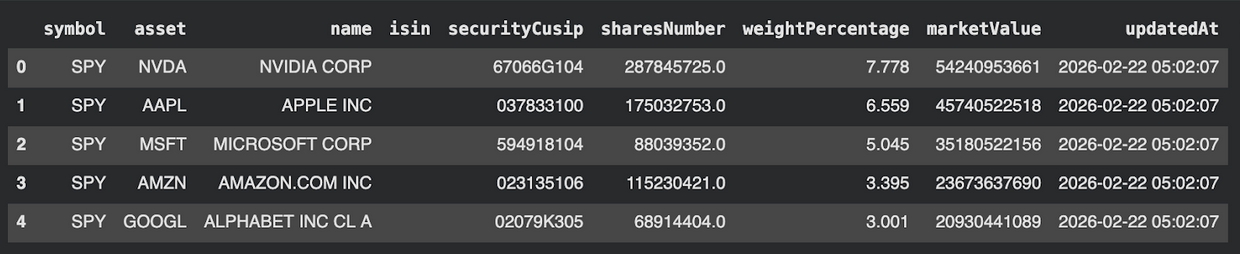
Portfolio weights must be numeric and non-null before aggregation. The analyzer performs defensive cleaning to ensure structural consistency.
|
# Ensure required columns exist required_cols = {"symbol", "weightPercentage"} missing_cols = required_cols - set(holdings_df.columns) if missing_cols: raise ValueError(f"Missing expected columns in holdings response: {missing_cols}") # Convert weight field holdings_df["weightPercentage"] = pd.to_numeric( holdings_df["weightPercentage"], errors="coerce" ) # Drop rows without symbol or weight holdings_df = holdings_df.dropna(subset=["symbol", "weightPercentage"]) # Ensure weights are positive holdings_df = holdings_df[holdings_df["weightPercentage"] > 0] holdings_df.head() |
Portfolio Weight Sanity Check
The total weight should approximate 100%, allowing for minor rounding differences.
|
total_weight = holdings_df["weightPercentage"].sum() print("Total Weight:", round(total_weight, 4)) |

This holdings dataset now provides a clean base structure for sector mapping. The next section associates each holding with its sector classification and aggregates portfolio exposure at the industry level.
Sector Mapping and Exposure Aggregation
The holdings dataset contains allocation weights but does not include sector classification. Sector metadata must therefore be retrieved separately for each holding symbol and merged back into the base dataset.
Retrieve Sector Classification
The Company Profile API provides sector information for each symbol.
|
def fetch_sector(symbol): profile_url = ( f"https://financialmodelingprep.com/stable/profile" f"?symbol={symbol}&apikey={API_KEY}" ) response = requests.get(profile_url) if response.status_code != 200: return None data = response.json() if isinstance(data, list) and len(data) > 0: return data[0].get("sector", None) return None |
Apply sector retrieval across holdings. For demonstration purposes, the first subset may be used to limit request volume.
|
# Limit number of holdings if needed for testing holdings_subset = holdings_df.copy() holdings_subset["sector"] = holdings_subset["asset"].apply(fetch_sector) holdings_subset.head() |

Defensive Handling of Missing Sectors
Some symbols may return None for sector classification. These must be retained but labeled clearly.
|
holdings_subset["sector"] = holdings_subset["sector"].fillna("Unknown") |
Aggregate Sector Exposure
Portfolio weight is aggregated by sector.
|
sector_exposure = ( holdings_subset .groupby("sector", as_index=False)["weightPercentage"] .sum() .sort_values("weightPercentage", ascending=False) ) sector_exposure |
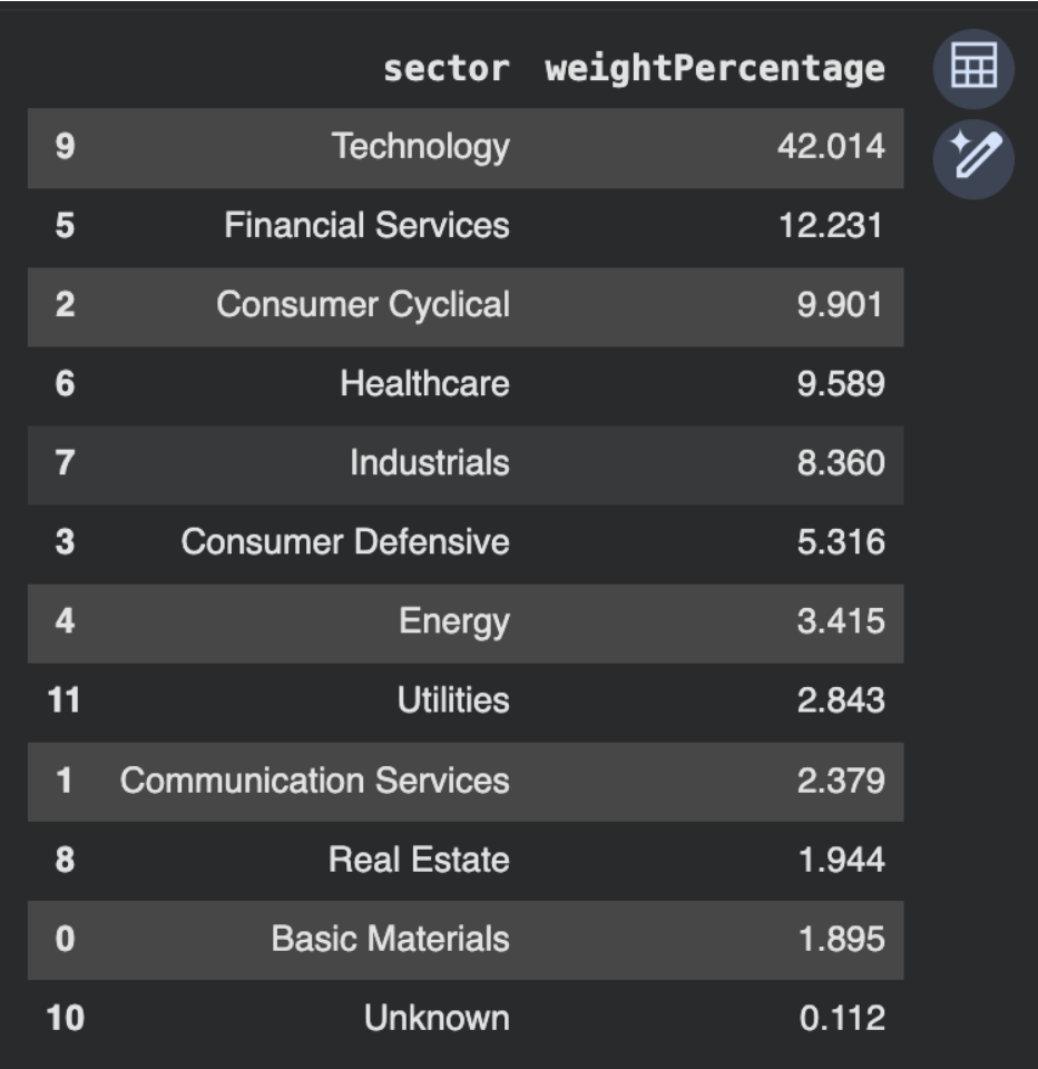
The sector distribution immediately highlights that SPY is not evenly balanced across industries. Technology accounts for approximately 42% of total portfolio weight, which is materially larger than any other sector allocation. Financial Services and Consumer Cyclical follow at significantly lower levels, while the remaining sectors each represent progressively smaller portions of the portfolio.
Although SPY holds hundreds of constituents, the exposure profile is structurally top-heavy due to capitalization weighting. This means the ETF's performance and volatility characteristics are meaningfully influenced by Technology-sector dynamics. The table therefore separates the perception of broad diversification from the reality of sector-driven concentration.
Exposure Sanity Check
Verify that aggregated sector exposure approximates total ETF weight.
|
sector_total = sector_exposure["weightPercentage"].sum() print("Sector Aggregated Weight:", round(sector_total, 4)) |

The analyzer now produces a clean sector exposure table derived directly from ETF holdings and sector metadata.
Sector Concentration Metrics and Structural Diagnostics
The sector exposure table describes allocation distribution. Structural diagnostics quantify concentration within that distribution. This section derives lightweight metrics from the existing sector_exposure dataframe without redefining prior objects.
Top Sector Weight
The largest sector allocation provides an immediate view of structural dominance.
|
top_sector_weight = sector_exposure["weightPercentage"].max() top_sector_name = sector_exposure.loc[ sector_exposure["weightPercentage"].idxmax(), "sector" ] print("Top Sector:", top_sector_name) print("Top Sector Weight:", round(top_sector_weight, 4)) |

In broad capitalization-weighted index ETFs, a top sector weight in the 20-30% range is relatively common, particularly when mega-cap industries dominate index composition. Once the leading sector exceeds roughly one-third of total allocation, sector concentration begins to materially influence ETF behavior. At that level, volatility patterns, drawdown sensitivity, and macro exposure can become increasingly tied to the dominant industry's performance cycle.
In this example, Technology represents approximately 42% of SPY's total weight, indicating that the ETF's risk profile is meaningfully shaped by Technology-sector dynamics despite its large number of individual holdings.
Top-N Sector Coverage
The proportion of capital concentrated in the largest sectors provides a broader concentration view.
|
top_n = 3 # configurable diagnostic top_n_weight = sector_exposure.head(top_n)["weightPercentage"].sum() print(f"Top {top_n} Sector Coverage:", round(top_n_weight, 4)) |

This metric shows how much of the portfolio is captured by the leading industry segments.
While the top sector weight highlights the single largest allocation, Top-3 Sector Coverage captures broader structural concentration across multiple dominant industries. If the leading three sectors collectively account for 60-70% of total portfolio weight, the ETF's behavior is largely shaped by a limited cluster of industry groups rather than by balanced cross-sector diversification.
In contrast, a more evenly diversified structure would distribute capital more uniformly across sectors, resulting in a lower Top-3 coverage figure. When this metric rises materially above half of total weight, sector-driven regime shifts and correlated industry drawdowns can have amplified effects on overall ETF performance.
Herfindahl-Style Concentration Index
A normalized Herfindahl-style metric provides a continuous concentration score.
|
# Convert percentage to decimal form sector_exposure["weight_decimal"] = sector_exposure["weightPercentage"] / 100 sector_exposure["weight_sq"] = sector_exposure["weight_decimal"] ** 2 herfindahl_index = sector_exposure["weight_sq"].sum() print("Herfindahl Concentration Index:", round(herfindahl_index, 6)) |

Values closer to zero indicate diversified exposure. Larger values reflect concentration.
The Herfindahl index provides a continuous measure of concentration, with values closer to zero indicating greater diversification. For broad capitalization-weighted index ETFs, values in the 0.10-0.20 range are common, reflecting multi-sector allocation with moderate concentration. As the index rises above approximately 0.25, structural dominance becomes more pronounced, and the ETF increasingly behaves like a sector-tilted allocation rather than a balanced industry mix.
Thematic or sector-specific ETFs often produce materially higher Herfindahl values, since capital is intentionally concentrated within a narrow segment of the market. In this example, a value near 0.22 suggests moderate concentration consistent with a broad index ETF that still exhibits meaningful sector weighting asymmetry.
Structural Diagnostic Summary
A compact summary consolidates the concentration diagnostics.
|
diagnostics_df = pd.DataFrame({ "Top Sector": [top_sector_name], "Top Sector Weight (%)": [round(top_sector_weight, 4)], "Top 3 Sector Coverage (%)": [round(top_n_weight, 4)], "Herfindahl Index": [round(herfindahl_index, 6)] }) diagnostics_df |

These diagnostics transform the exposure breakdown into measurable structural risk indicators.
Reading the Diagnostics Together
The three concentration metrics are most informative when interpreted collectively rather than in isolation. The Top Sector Weight identifies the single largest source of structural exposure, while Top-3 Sector Coverage captures broader clustering across dominant industries. The Herfindahl index complements these measures by translating the entire sector distribution into a continuous concentration score.
In this example, Technology's 42% allocation signals clear sector dominance. The fact that the top three sectors account for roughly 64% of total weight confirms that capital is clustered among a limited group of industries rather than evenly distributed. The Herfindahl value near 0.22 further supports this interpretation, indicating moderate concentration consistent with a broad index that is nevertheless meaningfully tilted toward specific sectors.
Taken together, the diagnostics show that SPY is diversified across many holdings but structurally influenced by a small set of dominant industries. This joint interpretation provides a clearer understanding of sector-driven risk than any single metric alone.
Sector Exposure Visualization and Output Structure
The sector exposure table represents the structural allocation across industries. This section formats the final exposure view and produces a clear visualization.
Final Sector Exposure Table
Ensure sorted order and clean formatting.
|
sector_exposure_final = sector_exposure[["sector", "weightPercentage"]].copy() sector_exposure_final = sector_exposure_final.sort_values( "weightPercentage", ascending=False ).reset_index(drop=True) sector_exposure_final["weightPercentage"] = sector_exposure_final["weightPercentage"].round(4) sector_exposure_final |
This table represents the ETF's industry allocation structure.
Sector Exposure Bar Chart
A simple bar chart improves interpretability without adding unnecessary complexity.
|
import matplotlib.pyplot as plt plt.figure() plt.bar(sector_exposure_final["sector"], sector_exposure_final["weightPercentage"]) plt.title("ETF Sector Exposure") plt.xlabel("Sector") plt.ylabel("Weight (%)") plt.xticks(rotation=45) plt.tight_layout() plt.show() |
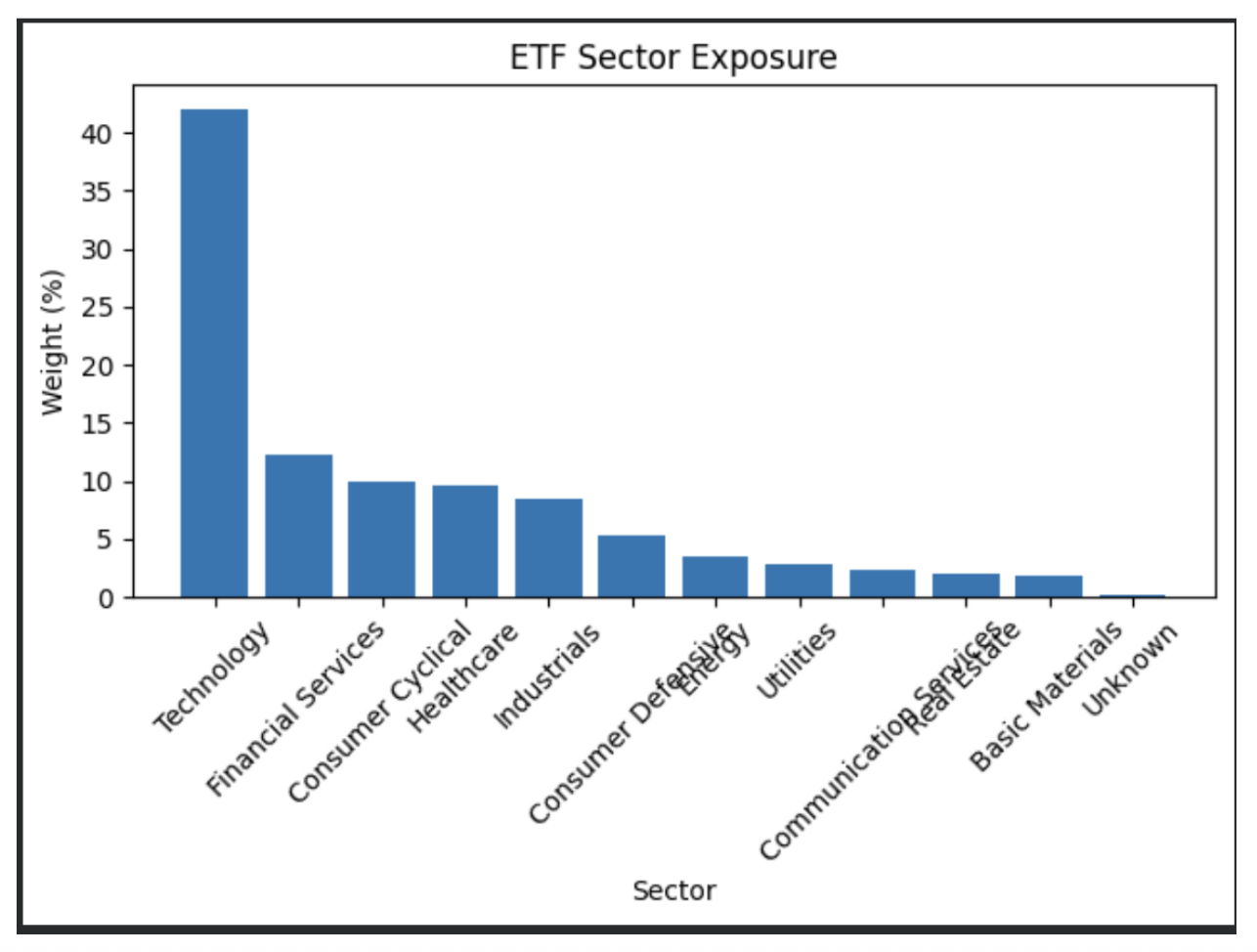
When concentration is high, the visualization clearly highlights dominance. When diversified, the distribution appears balanced across multiple sectors.
When This Framework Needs Adjustment
Although the Sector Exposure Analyzer provides a structured view of allocation concentration, certain conditions require careful interpretation.
Sector classification inconsistencies
Sector labels may differ across data providers or evolve over time as companies change business focus. Cross-market comparisons should account for potential taxonomy differences.
ETFs holding derivatives or cash equivalents
Some funds include futures, swaps, or cash positions that may not map cleanly to standard sector classifications. In such cases, reported exposure may understate or misrepresent effective economic allocation.
International ETFs with alternative industry standards
Global funds may rely on region-specific classification systems that do not align perfectly with U.S.-centric sector groupings. Direct comparisons across markets should consider these structural differences.
Rapid sector reclassification events
Corporate restructurings, spin-offs, or index methodology changes can materially alter sector exposure within a short period. Snapshot-based analysis should therefore be refreshed periodically to reflect current composition.
These considerations do not diminish the usefulness of the framework but reinforce the importance of validating sector mapping assumptions and ETF structure when interpreting concentration metrics.
Conclusion
This Sector Exposure Analyzer demonstrates how Financial Modeling Prep's stable ETF Holdings API and Company Profile API can be combined, with plan-level request capacity and data access limits shaping how efficiently the same workflow scales across multiple ETF universes. By retrieving portfolio weights, mapping each holding to its sector, and aggregating exposure, the workflow produces a clean sector breakdown and measurable concentration diagnostics. The result is a repeatable analytical framework that reveals structural bias and sector dominance within any ETF using directly sourced FMP data.