Build a Peer Set Generator That Actually Makes Comparable Peers

Comparable company analysis remains one of the most widely used valuation approaches in equity research, investment banking, and corporate finance. Its reliability, however, depends entirely on the quality of the selected peer group. In practice, many peer lists are constructed using only industry classification, which often results in structurally dissimilar companies being grouped together.

Industry alignment alone does not guarantee comparability. Two companies operating in the same sector may differ significantly in scale, capital intensity, profitability profile, growth trajectory, and valuation multiple structure. When these differences are ignored, the resulting valuation benchmarks become distorted and analytically weak.

A robust peer set must satisfy two layers of alignment:

• Structural similarity (industry, size, listing profile)
• Financial similarity (profitability, returns, valuation levels)

This article develops a systematic peer set generator using the financial data APIs provided by Financial Modeling Prep. The framework extracts structural attributes, constructs an initial candidate universe, integrates financial alignment metrics, and applies a quantitative similarity scoring model to produce a refined, valuation-ready peer group.

To demonstrate the workflow, we will use a large-cap semiconductor company as an example dataset. The framework, however, remains fully reusable across sectors and market capitalizations.

FMP APIs Used for Company Profiling, Screening, and Financial Comparison

• Company Profile: Provides sector, industry, exchange, and market capitalization used to define structural peer filters.
• Company Screener: Screens publicly listed companies using filters such as industry, sector, market cap range, country, exchange, and other constraints.
• Key Metrics TTM: Supplies trailing twelve month profitability, return, and performance metrics used for financial alignment.
• Financial Ratios TTM: Provides trailing twelve month valuation, efficiency, liquidity, and leverage ratios for comparability scoring.

Establishing Structural Filters for Peer Identification

A peer set must first satisfy structural alignment before any financial comparison begins. Structural alignment ensures that companies operate within the same economic framework and scale environment. Without this foundation, downstream financial comparisons lose analytical relevance.

To demonstrate the workflow, we will use a large-cap semiconductor company as an anchor example. The process, however, remains fully reusable across sectors.

Extracting Core Company Attributes

The first task is to retrieve sector, industry, exchange, and market capitalization. These attributes define the structural boundary of the peer universe.

We begin by pulling the company profile and storing only the fields required for screening.

How to Get Your API Key

To access Financial Modeling Prep's APIs, you need a valid API key.

Create an account using the official registration page.

After registration, your API key will be available in your dashboard. Replace "YOUR_API_KEY" in the code examples below with your personal key to authenticate requests.

Required Screening Fields

To construct a structurally aligned peer universe, we must first define the specific attributes that will drive the screening logic. These fields act as boundary constraints for the initial candidate pool.

From the company profile response, the following variables are required:

• Sector - Ensures high-level economic alignment
• Industry - Defines operational similarity
• Exchange - Maintains listing comparability
• Market Capitalization - Enables size proximity analysis

The code below extracts these attributes from the profile endpoint and stores them in a structured dictionary for downstream filtering.

import requests import pandas as pd API_KEY = "YOUR_API_KEY" BASE_URL = "https://financialmodelingprep.com/stable" symbol = "NVDA" # Anchor company for demonstration profile_url = f"{BASE_URL}/profile?symbol={symbol}&apikey={API_KEY}" profile_data = requests.get(profile_url).json() anchor_profile = { "symbol": symbol, "sector": profile_data[0]["sector"], "industry": profile_data[0]["industry"], "exchange": profile_data[0]["exchange"], "market_cap": profile_data[0]["marketCap"] } anchor_profile

This structured dictionary now holds the baseline characteristics that define comparability at a structural level.

Constructing a Market Capitalization Band

Industry alignment alone remains insufficient. Size materially influences capital structure, margin profile, and valuation multiples. A market capitalization band helps eliminate companies that operate in a materially different scale environment.

We construct a relative size band around the anchor company.

market_cap = anchor_profile["market_cap"] lower_bound = market_cap * 0.6 upper_bound = market_cap * 1.4 market_cap_range = { "min_market_cap": lower_bound, "max_market_cap": upper_bound } market_cap_range

This range defines acceptable size proximity. The bandwidth can be adjusted depending on the desired strictness of comparability.

At this stage, we have:

• Industry classification
• Exchange listing
• Market capitalization band

These structural filters will now be used to construct the initial candidate universe in the next section.

Constructing the Industry-Aligned Candidate Universe

Structural comparability begins with industry alignment. Size constraints are applied only after observing the distribution of companies within that industry.

Instead of restricting market capitalization at the API level, we first retrieve all listed companies operating within the same industry as the anchor entity. This ensures that the candidate universe is sufficiently broad and analytically stable.

Retrieving the Industry Universe

We query the Company Screener API using only industry and exchange filters derived earlier.

screener_url = ( f"{BASE_URL}/company-screener?" f"industry={anchor_profile['industry']}&" f"exchange={anchor_profile['exchange']}&" f"apikey={API_KEY}" ) industry_data = requests.get(screener_url).json()

This returns all publicly listed companies within the same industry classification on the same exchange as the anchor company.

Structuring the Industry Dataset

We now convert the response into a structured DataFrame and retain only the relevant structural attributes required for downstream filtering.

industry_df = pd.DataFrame(industry_data) industry_df = industry_df[ ["symbol", "companyName", "marketCap", "sector", "industry"] ] # Remove anchor company from the universe industry_df = industry_df[industry_df["symbol"] != symbol] industry_df.head()

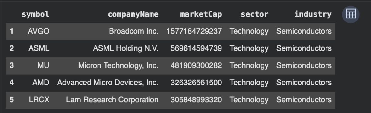
At this stage:

• The dataset represents the entire industry universe
• No size filtering has yet been applied
• The anchor company has been excluded from peer candidates

This guarantees that the candidate pool remains statistically meaningful, regardless of whether the anchor entity is small-cap, mid-cap, or mega-cap.

Evaluating Market Capitalization Distribution

Before applying size proximity filtering, we examine the market capitalization dispersion across the industry.

industry_df["marketCap"].describe()

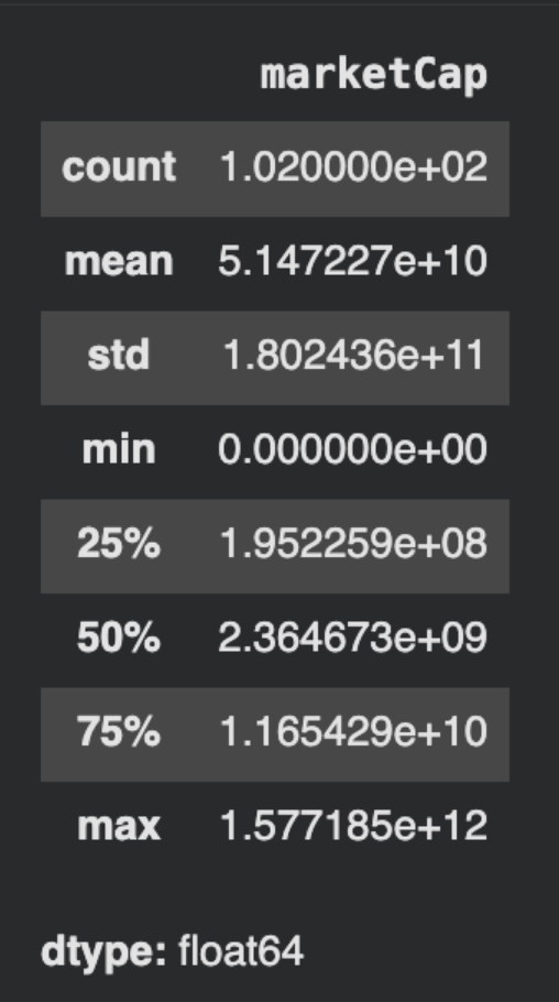
This summary provides visibility into:

• Industry size concentration
• Presence of extreme outliers
• Scale dispersion relative to the anchor

Rather than imposing an arbitrary size band at the API layer, size alignment will now be computed dynamically in the next section using relative distance measures.

This ensures that peer construction remains:

• Data-driven
• Scale-aware
• Robust across market capitalizations

Applying Market Capitalization Proximity Filtering

Industry alignment ensures economic similarity. Scale alignment ensures structural comparability.

Companies operating within the same industry may differ materially in market capitalization. Since valuation multiples, capital structure, and growth expectations are influenced by scale, market capitalization proximity becomes a necessary second filter.

Rather than applying an arbitrary band, we compute relative distance from the anchor company and retain the closest entities.

Computing Relative Market Capitalization Distance

We first calculate the absolute percentage difference between each candidate's market capitalization and the anchor company.

anchor_market_cap = anchor_profile["market_cap"] industry_df["marketCap_diff_pct"] = ( abs(industry_df["marketCap"] - anchor_market_cap) / anchor_market_cap ) industry_df.head()

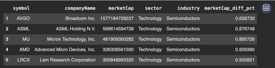
This metric represents relative size deviation.

• A value of 0.10 indicates 10% size difference.
• A value of 1.00 indicates 100% difference.

This approach avoids imposing rigid bands and instead measures actual structural proximity.

Ranking Companies by Size Similarity

We now rank companies by their relative distance and retain the closest candidates.

industry_df = industry_df.sort_values("marketCap_diff_pct") # Select top 15 closest companies by market cap proximity size_filtered_df = industry_df.head(15).reset_index(drop=True) size_filtered_df

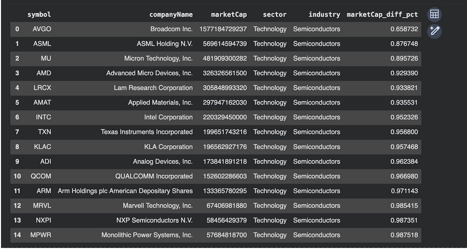
The number of retained candidates can be adjusted depending on desired strictness.

At this stage:

• Industry alignment is satisfied
• Scale proximity is quantified
• The candidate universe is reduced to structurally comparable entities

This filtered dataset now represents a size-aligned industry peer pool.

Although these companies represent the closest 15 peers by market capitalization within the semiconductor industry, the dispersion remains meaningful. The smallest deviation is approximately 65%, while many candidates exhibit size differences exceeding 90% relative to the anchor company.

This indicates that even within a tightly defined industry, scale concentration can vary significantly. Large-cap leaders often sit materially above the median industry size.

The ranking therefore ensures relative proximity, but it does not eliminate structural dispersion entirely. This reinforces the need to incorporate financial alignment metrics in the next stage to refine comparability beyond size alone.

Refining Peer Comparability Using Financial Alignment Metrics

The size-aligned universe now contains structurally similar companies. The next stage incorporates trailing twelve month capital efficiency and valuation indicators retrieved from the stable key metrics API.

These metrics allow peer selection to reflect operating performance and market valuation structure.

Integrating Capital Efficiency and Valuation Indicators

We retrieve key TTM metrics for each candidate and merge them into the working dataset.

def fetch_key_metrics(symbol): url = f"{BASE_URL}/key-metrics-ttm?symbol={symbol}&apikey={API_KEY}" response = requests.get(url).json() if isinstance(response, list) and len(response) > 0: return { "symbol": symbol, "roicTTM": response[0].get("returnOnInvestedCapitalTTM"), "roeTTM": response[0].get("returnOnEquityTTM"), "roaTTM": response[0].get("returnOnAssetsTTM"), "evToEBITDATTM": response[0].get("evToEBITDATTM"), "evToSalesTTM": response[0].get("evToSalesTTM") } return None metrics_data = [] for sym in size_filtered_df["symbol"]: data = fetch_key_metrics(sym) if data: metrics_data.append(data) metrics_df = pd.DataFrame(metrics_data) peer_df = size_filtered_df.merge(metrics_df, on="symbol", how="left") peer_df.head()

The dataset now includes:

• Market capitalization proximity
• Return on invested capital
• Return on equity
• Return on assets
• EV/EBITDA
• EV/Sales

These variables provide both performance and valuation alignment dimensions.

Designing a Quantitative Similarity Scoring Framework

Comparability must be measurable. Rather than applying manual cutoffs, we construct a similarity score based on normalized financial indicators and relative distance from the anchor company.

This converts the peer selection process into a ranking exercise grounded in observable metrics.

Preparing the Financial Feature Matrix

We first select the metrics that will drive similarity. These variables reflect capital efficiency and valuation structure.

# Select features for similarity scoring features = [ "roicTTM", "roeTTM", "roaTTM", "evToEBITDATTM", "evToSalesTTM", "marketCap_diff_pct" ] scoring_df = peer_df[["symbol"] + features].dropna().reset_index(drop=True) scoring_df.head()

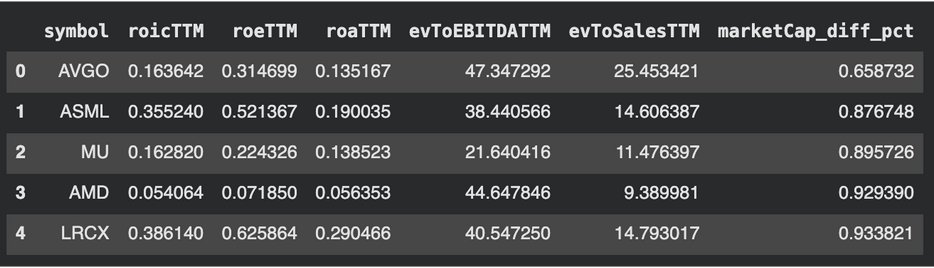
The dataset now contains only complete observations to ensure stability in scoring.

Normalizing Financial Indicators

The selected metrics operate on materially different numeric ranges. For example, ROIC may range between 5% and 40%, while EV/Sales can range from 2x to 25x or higher depending on growth expectations. Without normalization, valuation multiples would numerically dominate return metrics in a distance-based framework simply due to magnitude differences rather than analytical importance.

Normalization ensures that each variable contributes proportionally to the similarity score.

We apply min-max scaling to rescale all features between 0 and 1:

from sklearn.preprocessing import MinMaxScaler scaler = MinMaxScaler() scaled_values = scaler.fit_transform(scoring_df[features]) scaled_df = pd.DataFrame(scaled_values, columns=features) scaled_df["symbol"] = scoring_df["symbol"]

For those who prefer not to use external libraries, min-max scaling can also be implemented manually using:

scaled=(x−min)/(max−min)

This produces the same normalization effect while keeping the framework fully implementable with base Python and pandas. Each metric now ranges between 0 and 1 across the candidate set, ensuring a balanced contribution to the similarity calculation.

Computing the Similarity Score

We measure distance from the anchor company within the normalized feature space.

First, we extract the anchor company's scaled vector.

# Fetch anchor metrics anchor_metrics = fetch_key_metrics(symbol) anchor_vector = [ anchor_metrics.get("roicTTM"), anchor_metrics.get("roeTTM"), anchor_metrics.get("roaTTM"), anchor_metrics.get("evToEBITDATTM"), anchor_metrics.get("evToSalesTTM"), 0 # marketCap_diff_pct for anchor is zero ] # Normalize anchor vector using same scaler anchor_scaled = scaler.transform([anchor_vector])

Now compute Euclidean distance for each candidate.

import numpy as np scaled_features = scaled_df[features].values distances = np.linalg.norm(scaled_features - anchor_scaled, axis=1) scaled_df["similarity_score"] = distances # Lower distance = closer peer ranked_peers = scaled_df.sort_values("similarity_score") ranked_peers.head()

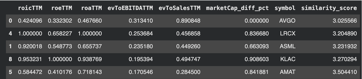
The similarity score reflects multidimensional proximity across:

• Scale
• Capital efficiency
• Valuation structure

Lower scores indicate stronger comparability.

How to Read the Similarity Ranking

The similarity score represents the Euclidean distance between each candidate company and the anchor company within the normalized feature space. Lower values indicate stronger multidimensional alignment across size, capital efficiency, and valuation structure.

In the example above, AVGO exhibits the lowest distance score, indicating the closest overall alignment to the anchor across the selected metrics. By contrast, AMAT displays the highest score among the top-ranked peers, suggesting comparatively greater dispersion in at least one dimension of profitability, valuation, or scale.

It is important to interpret these scores relatively rather than absolutely. A difference of 0.20-0.30 in similarity score reflects incremental divergence within the peer group, not structural dissimilarity. The ranking should therefore be viewed as a prioritization tool — identifying which companies warrant primary benchmarking focus before expanding to broader industry comparisons.

In practical valuation work, analysts typically concentrate on the top-ranked peers when constructing multiple ranges, target price sensitivity scenarios, or premium/discount diagnostics. The similarity framework formalizes this prioritization rather than relying on manual judgment.

Generating a Valuation-Ready Peer Comparison Output

The similarity ranking provides an ordered list of candidates. For valuation analysis, a concise and interpretable peer table is required. This table should contain only the most relevant comparability metrics and the top-ranked peers.

The objective is not to display every screened company, but to extract a focused subset suitable for benchmarking.

Selecting the Final Comparable Set

Traditional peer selection is often performed manually in spreadsheets. Analysts filter by industry, visually inspect market capitalization ranges, compare profitability metrics side-by-side, and iteratively remove outliers. While workable, this process is subjective, time-consuming, and difficult to reproduce consistently across companies.

The similarity framework above replaces that manual workflow with a fully systematic ranking process. Once the anchor symbol is defined, the model automatically screens, scores, and ranks comparable companies based on structural and financial alignment.

Simply replacing the anchor ticker (for example, from "NVDA" to "AMD" or "ASML") regenerates a new, valuation-ready peer set using the same methodology. This transforms peer construction from a one-off spreadsheet exercise into a repeatable analytical engine.

We now extract the top N peers based on similarity score. Lower scores represent stronger multidimensional alignment.

# Merge similarity score back to full dataset final_df = peer_df.merge( ranked_peers[["symbol", "similarity_score"]], on="symbol", how="inner" ) # Select top 5 most comparable companies top_peers = final_df.sort_values("similarity_score").head(5) top_peers[ [ "symbol", "marketCap", "roicTTM", "roeTTM", "evToEBITDATTM", "evToSalesTTM", "similarity_score" ] ]

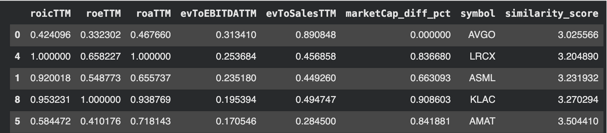
This table represents the finalized peer set suitable for:

• Relative valuation benchmarking
• Multiple comparison analysis
• Sector positioning review

Visual Comparison of Key Valuation Metrics

A visual representation strengthens interpretation. We compare EV/EBITDA across the selected peers.

import matplotlib.pyplot as plt plt.figure(figsize=(10, 6)) plt.bar( top_peers["symbol"], top_peers["evToEBITDATTM"] ) plt.title("EV/EBITDA Comparison Across Selected Peers") plt.ylabel("EV/EBITDA (TTM)") plt.xlabel("Company") plt.show()

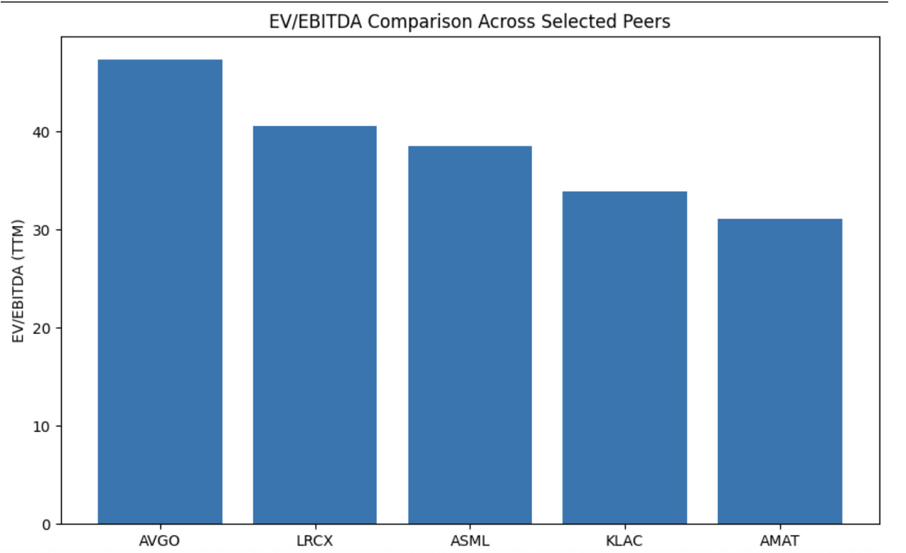
This chart highlights valuation dispersion within the refined peer group. Differences in multiples may reflect growth expectations, margin structure, or capital efficiency differences that can be further analyzed.

The dispersion across the peer group is economically meaningful. Broadcom (AVGO) trades at the highest EV/EBITDA multiple in the selected set, materially above Applied Materials (AMAT), which represents the lowest multiple in the group. The spread between the highest and lowest peer exceeds 15 multiple points, indicating substantial variation in market pricing despite structural and financial similarity.

Such dispersion may reflect differences in growth durability, margin expansion expectations, capital allocation strategy, or perceived competitive positioning. In practical valuation work, this output allows analysts to identify whether the anchor company trades at a premium or discount relative to its most comparable peers and to investigate the drivers behind that relative positioning.

At this stage, the peer generator has:

• Identified structurally aligned companies
• Quantified size proximity
• Integrated capital efficiency metrics
• Applied valuation filters
• Computed similarity scores
• Produced a ranked and valuation-ready peer set

The workflow is fully reusable. Replacing the anchor symbol automatically regenerates the peer group using the same framework.

When This Framework Needs Adjustment

While the similarity model provides a disciplined structure for peer selection, certain industry conditions may require modification. In cyclical sectors such as energy, materials, or semiconductors, trailing twelve-month profitability metrics can be temporarily distorted by earnings peaks or troughs, reducing their representativeness.

Companies with negative earnings or unstable return profiles may also produce misleading distance scores, particularly when valuation multiples become extreme or undefined. In some cases, key metrics may be missing or incomplete, requiring alternative indicators or adjusted feature selection.

Highly capital-intensive industries may further demand sector-specific normalization, as scale and leverage dynamics can behave differently from asset-light businesses. The framework is therefore best viewed as a structured baseline that can be adapted to industry context rather than a rigid, one-size-fits-all solution.

Conclusion

A reliable comparable analysis begins with disciplined peer selection. Industry labels alone do not ensure analytical validity. Scale proximity, capital efficiency, and valuation structure must be considered together.

This framework demonstrates how to construct a systematic peer set generator using Financial Modeling Prep's stable APIs, with plan-level request capacity determining how broadly you can scale the same workflow across larger universes.

The methodology remains fully reusable across sectors and market capitalizations. Replacing the anchor symbol automatically rebuilds the peer universe, enabling consistent and scalable comparable company analysis.