Build an Earnings Revision Pressure Signal (Estimate Drift Monitor)

Earnings expectations evolve continuously as analysts update models, adjust assumptions, and react to new information. These incremental changes often precede visible shifts in reported fundamentals. In practice, sustained upward revisions frequently emerge ahead of positive earnings surprises, while persistent downward adjustments tend to signal growing caution before disappointments. Monitoring this estimate drift provides a structured way to observe expectation momentum before results are released. Rather than reacting to the earnings announcement itself, investors can use revision pressure to assess whether risk is building, positioning is becoming crowded, or consensus is stabilizing ahead of the event.

This article develops an Earnings Revision Pressure signal by tracking changes in forward EPS consensus over time. The objective is not to construct a production trading system, but to demonstrate how Financial Modeling Prep's stable analyst estimate data can be transformed into a compact monitoring framework.

The workflow builds a time-stamped estimate ledger, measures drift between successive observations, and converts those revisions into a single interpretable pressure score. The result is a repeatable signal that reflects whether expectations are strengthening, deteriorating, or stabilizing ahead of the next reporting cycle.

The following section outlines the specific FMP APIs used to construct this monitoring structure.

FMP APIs Used

This use case relies on two stable Financial Modeling Prep endpoints. One provides forward-looking consensus estimates, and the other anchors the monitoring window around earnings events.

• Financial Estimates API:Retrieves forward-period analyst consensus data, including EPS and revenue aggregates such as epsLow, epsAvg, epsHigh, and related fields.
• Earnings Calendar API: Provides upcoming and historical earnings event dates along with estimated and actual EPS values.

How to Get Your API Key

To access Financial Modeling Prep's APIs, you need a valid API key.

Create an account using the official registration page.

After registration, your API key will be available in your dashboard. Replace "YOUR_API_KEY" in the code examples below with your personal key to authenticate requests.

Consensus Estimate Snapshots as a Time-Stamped Dataset

The Financial Estimates endpoint returns forward-period consensus values keyed by fiscal period date. It does not provide a historical revision timeline.

Because the API reflects the current consensus state rather than a versioned history of prior estimate changes, historical drift must be captured locally over time. Snapshot storage is therefore not optional in a monitoring framework. Without repeated observations of the same fiscal period, it is not possible to quantify how expectations evolved between points in time.

A drift monitor therefore requires repeated observations stored with a local timestamp. This section constructs a snapshot dataset that can be extended over time.

The example below uses a single symbol for demonstration. The variable flow remains consistent throughout the article.

import requests import pandas as pd from datetime import datetime API_KEY = "YOUR_API_KEY" symbol = "NVDA" period = "quarter" # or "annual" estimates_url = ( f"https://financialmodelingprep.com/stable/analyst-estimates" f"?symbol={symbol}&period={period}&apikey={API_KEY}" ) response = requests.get(estimates_url) if response.status_code != 200: raise Exception(f"API request failed: {response.status_code} - {response.text}") raw_data = response.json() # Validate structure before selecting fields if not isinstance(raw_data, list) or len(raw_data) == 0: raise ValueError("No estimate data returned for the symbol.") estimates_df = pd.DataFrame(raw_data) # Inspect available columns print(estimates_df.columns)

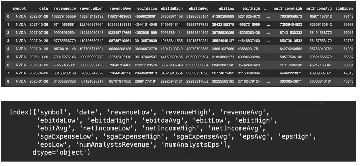
The monitor focuses on the next reporting period. The dataset is sorted chronologically, and the nearest future fiscal period is selected.

# Ensure proper date parsing estimates_df["date"] = pd.to_datetime(estimates_df["date"], errors="coerce") # Drop invalid dates estimates_df = estimates_df.dropna(subset=["date"]) # Sort by fiscal period estimates_df = estimates_df.sort_values("date") today = pd.Timestamp.today() # Select the nearest future fiscal period target_period = estimates_df[estimates_df["date"] >= today].head(1) if target_period.empty: raise ValueError("No forward fiscal period found in estimate data.") snapshot = target_period[["date", "epsLow", "epsAvg", "epsHigh"]].copy() # Attach observation timestamp snapshot["observed_at"] = datetime.utcnow() snapshot

The full analyst estimate response typically returns multiple forward fiscal periods, often covering several upcoming quarters and, in some cases, annual projections. Each row corresponds to a specific fiscal period and contains consensus aggregates such as epsLow, epsAvg, and epsHigh derived from contributing analysts.

The snapshot constructed above isolates the nearest forward fiscal period and captures its consensus state at a specific observation timestamp. Structurally, this row represents a point-in-time record of market expectations for the upcoming reporting cycle. When collected repeatedly over time, these point-in-time records form the basis for measuring revision drift.

This snapshot dataframe represents a single observation of consensus expectations for the next fiscal period. In a monitoring setup, this structure would be appended to a persistent store at regular intervals.

Drift and Revision Metrics on the Snapshot Ledger

A single snapshot does not provide revision information. Drift emerges only when multiple observations of the same fiscal period are compared. The snapshot structure constructed earlier therefore becomes a ledger once additional observations are appended over time.

For demonstration purposes, assume multiple snapshots have been collected for the same fiscal period and stored in a dataframe named ledger_df. The structure mirrors the previously created snapshot dataframe.

# Example structure of a revision ledger # In practice, snapshots are appended over time ledger_df = pd.concat([snapshot]).copy()

At this stage, ledger_df contains only a single snapshot and therefore does not yet exhibit any revision behavior. The structure is defined intentionally as a ledger placeholder so that additional observations can be appended over time. Meaningful drift metrics emerge only once multiple snapshots of the same fiscal period are stored with different observation timestamps.

# Ensure correct types ledger_df["observed_at"] = pd.to_datetime(ledger_df["observed_at"], errors="coerce") ledger_df = ledger_df.sort_values("observed_at")

In a live monitor, ledger_df would contain several rows for the same fiscal date, each with a different observed_at timestamp.

Revision Delta

The first measure is the net change in consensus EPS between consecutive observations.

ledger_df["eps_revision"] = ledger_df["epsAvg"].diff()

This captures the absolute revision between snapshots. A positive value indicates upward estimate revision. A negative value indicates downward revision.

The magnitude of the revision should be interpreted relative to the EPS level itself. For a company with forward EPS near $1.00, a $0.05 adjustment represents a 5% change and may be economically meaningful. For a company with forward EPS near $10.00, the same absolute change is proportionally smaller. Absolute deltas therefore provide directional information, but proportional context is often necessary when comparing across symbols or evaluating materiality.

Revision Rate

The rate normalizes the revision by elapsed time between observations.

ledger_df["days_between"] = ledger_df["observed_at"].diff().dt.days ledger_df["revision_rate"] = ledger_df["eps_revision"] / ledger_df["days_between"]

This prevents large revisions over long gaps from appearing equivalent to sharp short-term changes.

However, very small day gaps between observations can mechanically inflate the revision_rate value, so monitoring frequency should remain consistent to avoid overstating short-interval adjustments.

Dispersion Shift (Optional Stability Measure)

When epsLow and epsHigh are available, estimate dispersion can be monitored.

ledger_df["dispersion"] = ledger_df["epsHigh"] - ledger_df["epsLow"] ledger_df["dispersion_change"] = ledger_df["dispersion"].diff()

Narrowing dispersion suggests increasing analyst agreement. Widening dispersion indicates uncertainty.

Defensive Handling for Sparse Data

Revision metrics require at least two observations. The monitor must validate ledger depth before computing signals.

if ledger_df.shape[0] < 2: print("Insufficient snapshots to compute revision metrics.")

With revision delta, rate, and dispersion changes defined, the next section integrates these components into a consolidated Earnings Revision Pressure signal.

Add a Simulated Prior Snapshot (Demonstration Only)

We create a prior observation with an earlier observed_at timestamp and slightly different consensus EPS.

# Simulated prior snapshot (for demonstration) prior_snapshot = snapshot.copy() prior_snapshot["observed_at"] = prior_snapshot["observed_at"] - pd.Timedelta(days=14) prior_snapshot["epsAvg"] = prior_snapshot["epsAvg"] - 0.05 prior_snapshot["epsLow"] = prior_snapshot["epsLow"] - 0.04 prior_snapshot["epsHigh"] = prior_snapshot["epsHigh"] - 0.06 # Build ledger with two observations ledger_df = pd.concat([prior_snapshot, snapshot]).sort_values("observed_at").reset_index(drop=True)

Now recompute metrics:

ledger_df["eps_revision"] = ledger_df["epsAvg"].diff() ledger_df["days_between"] = ledger_df["observed_at"].diff().dt.days ledger_df["revision_rate"] = ledger_df["eps_revision"] / ledger_df["days_between"] ledger_df["dispersion"] = ledger_df["epsHigh"] - ledger_df["epsLow"] ledger_df["dispersion_change"] = ledger_df["dispersion"].diff() ledger_df

Earnings Revision Pressure Signal Construction

Revision metrics are now available at the ledger level. This section consolidates them into a single interpretable pressure score. The objective is to summarize directional momentum in consensus expectations without introducing unnecessary complexity.

The signal uses three components:

• Net EPS revision
• Revision rate (time-normalized)
• Dispersion change (uncertainty adjustment)

Upward revisions increase pressure positively. Widening dispersion reduces confidence in that pressure.

Component Normalization

To keep the score comparable across symbols, the revision is scaled relative to the absolute EPS level.

# Avoid division by zero ledger_df["eps_level"] = ledger_df["epsAvg"].replace(0, pd.NA) ledger_df["revision_pct"] = ledger_df["eps_revision"] / ledger_df["eps_level"]

This converts the raw revision into a proportional change.

Core Pressure Score

The pressure score combines proportional revision and revision rate. Dispersion widening acts as a penalty.

# Replace missing values defensively ledger_df["revision_pct"] = ledger_df["revision_pct"].fillna(0) ledger_df["revision_rate"] = ledger_df["revision_rate"].fillna(0) ledger_df["dispersion_change"] = ledger_df["dispersion_change"].fillna(0) # Pressure score construction ledger_df["revision_pressure"] = ( ledger_df["revision_pct"] * 0.6 + ledger_df["revision_rate"] * 0.3 - ledger_df["dispersion_change"] * 0.1 )

The weights are deliberately simple. The goal is interpretability rather than optimization.

The weights are deliberately simple and heuristic. Proportional revision receives the highest weight because it reflects the economic significance of consensus change relative to EPS level. The revision rate contributes directional momentum, while dispersion change acts as a confidence adjustment. The objective is interpretability rather than optimization, allowing the signal components to remain transparent and structurally intuitive.

Latest Signal Snapshot

Only the most recent observation represents the active monitoring signal.

current_signal = ledger_df.tail(1)[[ "date", "observed_at", "eps_revision", "revision_rate", "dispersion_change", "revision_pressure" ]] current_signal

• A positive revision_pressure indicates strengthening consensus expectations.
• A negative value reflects deteriorating forward sentiment.
• A near-zero value indicates stability.

Because the score is constructed from proportional revision and time-normalized momentum, its magnitude should be interpreted relative to recent observations for the same symbol. In practice, small values near zero typically reflect incremental estimate adjustments or stable consensus conditions. Sustained positive readings that are materially larger than recent baseline fluctuations suggest strengthening upward revision pressure, while persistently negative readings indicate broad-based downward adjustment in expectations.

There is no universal threshold for what qualifies as “strong” pressure, since EPS levels and revision frequency vary across companies. The signal is therefore most informative when evaluated as a directional and relative indicator rather than a fixed-rule trigger.

Monitor Output and Earnings Context Alignment

The revision pressure score becomes meaningful when evaluated alongside earnings timing. This section aligns the computed signal with the upcoming earnings date and presents a compact monitoring view.

Retrieve Earnings Event Context

The stable earnings calendar response can contain only historical rows, and EPS fields may be missing for some events. The logic below selects the next earnings date if available. Otherwise, it falls back to the latest available event and retains nullable EPS values.

import requests import pandas as pd import matplotlib.pyplot as plt # Pull earnings calendar earnings_url = ( f"https://financialmodelingprep.com/stable/earnings-calendar" f"?symbol={symbol}&apikey={API_KEY}" ) earnings_response = requests.get(earnings_url) if earnings_response.status_code != 200: raise Exception(f"Earnings API request failed: {earnings_response.status_code} - {earnings_response.text}") earnings_data = earnings_response.json() if not isinstance(earnings_data, list) or len(earnings_data) == 0: raise ValueError("No earnings calendar data returned for the symbol.") earnings_df = pd.DataFrame(earnings_data) # Validate expected columns exist before selection required_cols = {"date", "epsEstimated", "epsActual", "lastUpdated"} missing = required_cols - set(earnings_df.columns) if missing: raise ValueError(f"Missing expected columns in earnings response: {missing}") # Parse and clean dates earnings_df["date"] = pd.to_datetime(earnings_df["date"], errors="coerce") earnings_df = earnings_df.dropna(subset=["date"]).sort_values("date") earnings_df["date_norm"] = earnings_df["date"].dt.normalize() today = pd.Timestamp.now().normalize() # Prefer future earnings if present, else fall back to latest historical next_earnings = earnings_df[earnings_df["date_norm"] > today].head(1) if next_earnings.empty: anchor_earnings = earnings_df[earnings_df["date_norm"] <= today].tail(1) anchor_type = "latest" else: anchor_earnings = next_earnings anchor_type = "next" anchor_earnings_view = anchor_earnings[["date", "epsEstimated", "epsActual", "lastUpdated"]].copy() anchor_earnings_view["anchor_type"] = anchor_type

This provides contextual alignment between the consensus revision pressure and the next reporting event.

The interpretive value of revision pressure typically increases as the earnings date approaches. When consensus adjustments occur within a compressed pre-announcement window, they often reflect higher analyst conviction or late-cycle information updates. By contrast, revisions occurring far from the reporting date may represent gradual model recalibration rather than immediate sentiment shifts. Monitoring the proximity between observation timestamp and earnings anchor therefore helps distinguish structural drift from event-driven pressure.

Compact Monitoring Table

The monitor table retains the signal metrics from current_signal and appends the earnings anchor as contextual metadata. No merge is performed on dates.

monitor_df = current_signal.copy() monitor_df["earnings_anchor_type"] = anchor_earnings_view["anchor_type"].iloc[0] monitor_df["earnings_anchor_date"] = anchor_earnings_view["date"].iloc[0] monitor_df["earnings_epsEstimated"] = anchor_earnings_view["epsEstimated"].iloc[0] monitor_df["earnings_epsActual"] = anchor_earnings_view["epsActual"].iloc[0] monitor_df["earnings_lastUpdated"] = anchor_earnings_view["lastUpdated"].iloc[0] monitor_df["earnings_eps_available"] = ( monitor_df["earnings_epsEstimated"].notna() | monitor_df["earnings_epsActual"].notna() ) monitor_df

Operationally, this table functions as a compact monitoring record for the current earnings cycle. In a production setting, it could be generated on a scheduled basis—such as daily or weekly—and stored for a defined universe of symbols. Analysts may use it to track revision pressure across a watchlist, flag names exhibiting accelerating upward or downward drift, or integrate it into broader portfolio risk dashboards. Because the structure isolates both the pressure score and earnings timing metadata, it supports systematic screening rather than ad hoc inspection.

Visual Drift Representation

A minimal visualization shows how the consensus EPS series evolved across observation timestamps and how the consolidated pressure score behaves.

# Ensure the ledger is ordered for plotting plot_df = ledger_df.sort_values("observed_at").copy() plt.figure() plt.plot(plot_df["observed_at"], plot_df["epsAvg"]) plt.title("Consensus EPS Drift (Snapshot Ledger)") plt.xlabel("Observation Timestamp") plt.ylabel("EPS Average") plt.xticks(rotation=45) plt.tight_layout() plt.show() plt.figure() plt.plot(plot_df["observed_at"], plot_df["revision_pressure"]) plt.title("Earnings Revision Pressure (Snapshot Ledger)") plt.xlabel("Observation Timestamp") plt.ylabel("Revision Pressure Score") plt.xticks(rotation=45) plt.tight_layout() plt.show()

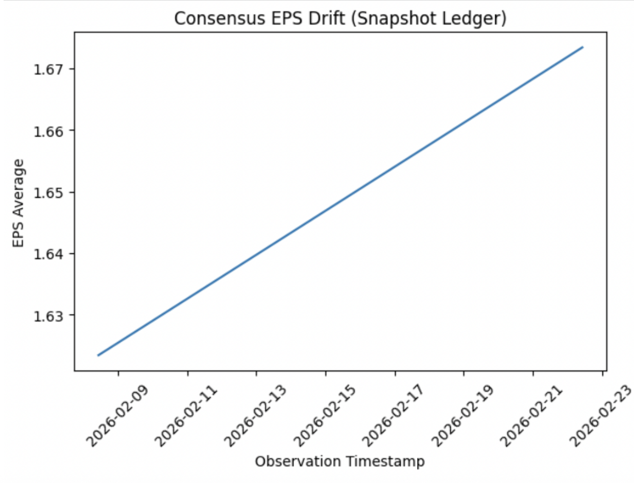
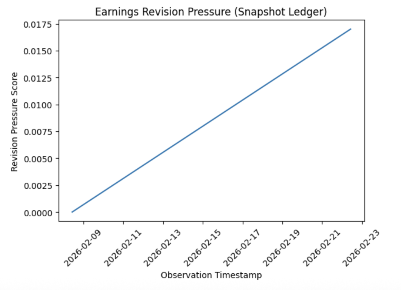
This chart illustrates whether consensus expectations are trending upward, downward, or flattening as the earnings date approaches.

In practice, a sustained upward drift in consensus EPS accompanied by stable or narrowing dispersion often precedes positive earnings surprises, as analysts incrementally adjust expectations higher ahead of results. Conversely, persistent downward revisions or widening dispersion may signal deteriorating confidence before a negative outcome. While revision pressure does not guarantee surprise direction, consistent directional patterns in the ledger visualization provide early evidence of expectation momentum building into the reporting date.

This monitor output completes the connected workflow: the estimate ledger generates revision metrics and a consolidated pressure score, while the earnings calendar provides a nullable timing anchor that remains informative even when EPS fields are not available.

When This Signal Can Mislead

Like any estimate-based metric, revision pressure should be interpreted within structural context. Several conditions can distort or overstate the signal:

Low analyst coverage

Companies followed by only a small number of analysts may exhibit exaggerated revisions when a single contributor updates forecasts. In these cases, dispersion and revision magnitude may reflect limited sample size rather than broad sentiment change.

Thin estimate update frequency

If estimates are updated infrequently, long gaps between observations can compress multiple adjustments into a single revision event. This may produce abrupt shifts that reflect accumulated changes rather than sudden information flow.

Sudden large revisions after long inactivity

Large absolute revisions following extended quiet periods can inflate proportional metrics and revision rates. Without consistent monitoring cadence, interpretation of velocity becomes less reliable.

Structural upward drift in high-growth names

High-growth companies often experience persistent upward estimate revisions as business scale expands. In such cases, steady positive pressure may reflect structural growth trends rather than incremental surprise risk into a specific earnings event.

These conditions do not invalidate the signal, but they reinforce the importance of evaluating revision pressure alongside coverage depth, update cadence, and broader company context.

Conclusion

This article demonstrated how to construct an Earnings Revision Pressure signal using Financial Modeling Prep's stable Analyst Estimates API and Earnings Calendar API. The workflow captures forward EPS consensus snapshots, measures revision drift across observation timestamps, and converts those changes into a structured pressure score. Because the signal is derived directly from FMP estimate aggregates and aligned to the earnings calendar, it remains data-consistent and resilient to incomplete event-level fields.

The result is a disciplined monitoring framework that transforms raw analyst estimate updates into a clear, repeatable indicator of expectation momentum. When deployed across a broader coverage universe, the frequency of snapshot collection and historical depth of stored revisions will depend on the data access tier supporting the monitoring workflow.