Filing Delta Monitor: Tracking What Changed Between Institutional Filings

Institutional investors disclose their portfolio holdings through 13F filings, offering a structured view of how capital is allocated across securities. These filings are widely used by analysts to track fund positioning, identify conviction bets, and monitor exposure across sectors. However, a single filing represents only a snapshot in time and does not capture how a portfolio is evolving.
In practice, the real signal lies in comparing filings across periods. Changes in holdings—such as new positions, exits, or adjustments in position size—often reflect shifts in conviction, portfolio rebalancing, or strategic repositioning. Without a systematic way to track these changes, it becomes difficult to extract actionable insights from raw filing data.
In this article, we build a Filing Delta Monitor that compares two institutional filings and identifies what has changed between them. Using Financial Modeling Prep's Filings Extract API and Python, we construct a data-driven framework to classify position-level changes and quantify capital allocation shifts across reporting periods. More importantly, this framework goes beyond simple comparison by systematically detecting shifts in institutional conviction, making the output usable as a signal within broader research workflows.
Financial Modeling Prep API Used
Filings Extract API: This endpoint provides structured holdings data that can be directly compared across different quarters. By retrieving filings for two reporting periods using the same CIK, we can align positions and compute changes in holdings, enabling a clean and reproducible delta analysis.
How to Get Your API Key
To access Financial Modeling Prep's APIs, you need a valid API key.
Create an account using the official registration page.
After registration, your API key will be available in your dashboard. Replace "YOUR_API_KEY" in the code examples below with your personal key to authenticate requests.
Framework Definition: Building the Filing Delta Monitor
Before writing the code, we need to define how the monitor will work. The goal is to compare two institutional filings for the same investor and convert raw holdings data into a structured change-detection framework.
This framework focuses on position-level movement across reporting periods. Instead of treating each filing as a static snapshot, it measures how holdings appear, disappear, or change in size between quarters. In practice, this enables analysts to track capital rotation, identify emerging positions, and detect early shifts in institutional sentiment across portfolios.
Comparing Two Reporting Periods
The analysis begins by selecting two filings for the same institution using a common CIK. Each filing represents a different quarter and contains position-level data such as symbol, shares, and market value.
Using the same institution across two reporting periods makes the comparison consistent. It ensures that any detected change reflects portfolio movement rather than differences across filers.
Aligning Positions Across Filings
The next step is to align holdings across both periods using the symbol as the comparison key. This makes it possible to track the same security from one filing to the next.
After alignment, the dataset shows whether a holding exists in both filings or only in one of them. That structure is necessary before any classification logic can be applied.
Classifying Position Changes
Once the holdings are aligned, each position can be interpreted based on its presence and its change in share count. A position that appears only in the latest filing is treated as a new addition, while one missing from the latest filing is treated as an exit.
If the position exists in both filings, the share counts are compared to determine whether the institution increased, reduced, or maintained that holding. This turns raw filing data into a usable portfolio-change signal.
Measuring the Magnitude of Change
Classification alone is not enough, because not all changes carry the same weight. A small reduction in shares and a large allocation shift should not be interpreted in the same way.
To address this, the monitor also calculates the change in shares and the change in position value between the two filings. These metrics help separate minor rebalancing activity from stronger conviction shifts.
Constructing the Final Analytical Dataset
The final output combines aligned holdings, delta classification, and change magnitude into one structured dataset. Each row captures how a specific position changed between the two filings.
This final dataset forms the core of the Filing Delta Monitor. It gives analysts a clean way to study how institutional portfolios evolve across reporting periods.
Python Implementation: Building the Filing Delta Monitor
This section translates the framework into a reproducible Python workflow. We begin by retrieving holdings for two reporting periods, then align the positions, calculate filing-level changes, and build the final delta monitor output.
Each step adds one part of the analytical pipeline, moving from raw API response to an interpretable comparison table.
Step 1: Retrieve Filing Data for Two Reporting Periods
To begin, we select an institutional investor using its CIK (Central Index Key). In this example, we use:
- CIK: 0001388838
This CIK corresponds to an institutional filer whose 13F holdings are available across multiple quarters. We retrieve filings for two consecutive quarters to enable comparison.
|
import requests import pandas as pd API_KEY = "YOUR_API_KEY" cik = "0001388838" # Example institution def fetch_filing(cik, year, quarter): url = "https://financialmodelingprep.com/stable/institutional-ownership/extract" params = { "cik": cik, "year": year, "quarter": quarter, "apikey": API_KEY } response = requests.get(url, params=params) data = response.json() return pd.DataFrame(data) # Fetch two quarters df_prev = fetch_filing(cik, 2023, 2) df_curr = fetch_filing(cik, 2023, 3) print("Previous Filing Shape:", df_prev.shape) print("Current Filing Shape:", df_curr.shape) print("\nColumns:") print(df_curr.columns.tolist()) print("\nSample Current Filing:") print(df_curr.head()) |
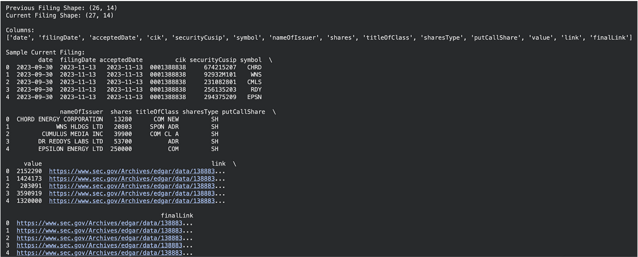
At this stage, we are primarily verifying the number of positions, available symbols, and key fields such as shares and value, since this consistent structure is what enables direct comparison across reporting periods.
The code retrieves position-level holdings for two reporting periods using the Filings Extract API. Each API call returns a list of securities held by the institution for a given quarter, which is converted into a pandas DataFrame.
From the output, the previous filing contains 26 positions, while the current filing contains 27 positions. Both datasets share the same structure, with key columns such as symbol, shares, and value, along with additional metadata like issuer name and filing dates.
This confirms that the API provides consistent, structured data across quarters, making it suitable for direct comparison.
Interpretation
The difference in the number of positions confirms that at least one addition or exit occurred between the two filings. Specifically, the increase from 26 to 27 positions suggests that at least one new position has been added in the latest filing.
Since both filings contain identical column structures, we can reliably align holdings using the symbol field. This ensures that any detected changes in shares or value reflect actual portfolio movement rather than inconsistencies in the dataset.
With the data successfully retrieved and validated, we can now move to preparing clean comparison datasets for delta computation.
Step 2: Prepare Clean Comparison DataFrames
Before comparing the two filings, we need to clean and standardize the datasets. The raw API response contains multiple fields, but for delta analysis, only a subset is required.
We focus on the core attributes that define each position:
- symbol → Unique identifier
- shares → Position size
- value → Capital allocation
We also rename columns to distinguish between the previous and current filings, which simplifies comparison in later steps.
|
# Select relevant columns df_prev_clean = df_prev[['symbol', 'shares', 'value']].copy() df_curr_clean = df_curr[['symbol', 'shares', 'value']].copy() # Rename columns for clarity df_prev_clean.rename(columns={ 'shares': 'shares_prev', 'value': 'value_prev' }, inplace=True) df_curr_clean.rename(columns={ 'shares': 'shares_curr', 'value': 'value_curr' }, inplace=True) print("Previous Filing (Cleaned):") print(df_prev_clean.head()) print("\nCurrent Filing (Cleaned):") print(df_curr_clean.head()) |
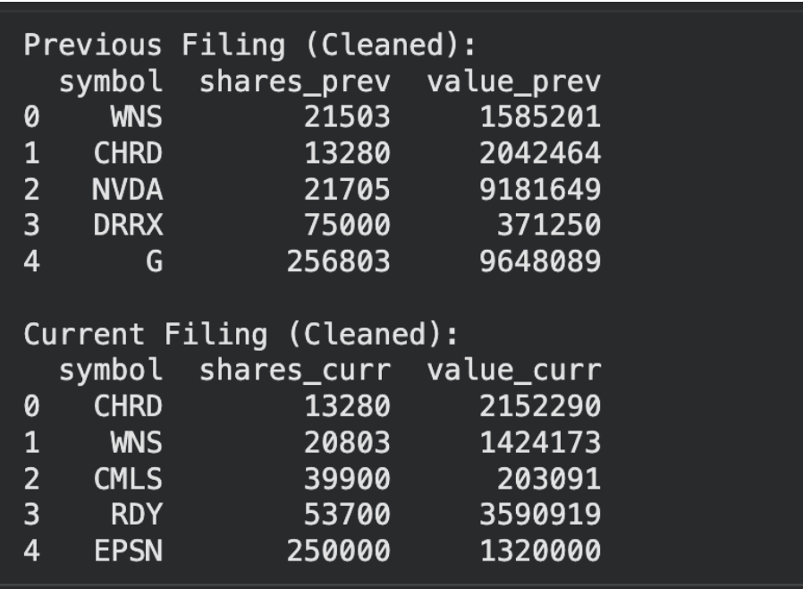
At this stage, the datasets isolate the core variables required for delta computation—shares and value—while removing unnecessary fields that could introduce noise before alignment.
This step standardizes both filings by retaining only the essential fields required for comparison: symbol, shares, and value. Removing additional metadata keeps the analysis focused and reduces unnecessary complexity.
The columns are renamed to clearly distinguish between the previous and current filings. This ensures that when the datasets are merged in the next step, each value can be correctly attributed to its respective reporting period.
Interpretation
The cleaned datasets show that both filings are now aligned in structure and ready for direct comparison. Each row represents a position with clearly separated metrics for the previous and current periods.
Even at this stage, early signals are visible. For example, WNS appears in both filings with a slight reduction in shares, indicating a potential trimming of the position. CHRD is also present in both filings, suggesting continuity in holding, while new symbols such as CMLS, RDY, and EPSN appear in the current filing but not in the sample of the previous one, hinting at new additions.
These observations are preliminary, as the datasets are not yet fully aligned across all positions. A complete view of additions, exits, and changes will emerge after merging both filings in the next step.
Step 3: Align Holdings Across Filings
With both datasets cleaned and standardized, the next step is to align positions across the two filings. This allows us to compare holdings at the security level and identify whether a position exists in one or both periods.
We perform an outer merge on the symbol column to ensure that all positions are retained. This includes positions that appear only in the previous filing, only in the current filing, or in both.
|
# Merge datasets on symbol df_merged = pd.merge( df_prev_clean, df_curr_clean, on="symbol", how="outer" ) # Fill missing values with 0 for comparison df_merged[['shares_prev', 'value_prev']] = df_merged[['shares_prev', 'value_prev']].fillna(0) df_merged[['shares_curr', 'value_curr']] = df_merged[['shares_curr', 'value_curr']].fillna(0) print("Merged Dataset:") print(df_merged.head(10)) |
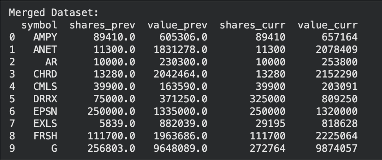
This merged table enables direct comparison of position presence, changes in position size, and shifts in capital allocation across reporting periods.
In this step, both filings are merged using an outer join on the symbol column. This ensures that all positions from both periods are included, regardless of whether they exist in one filing or both.
Missing values are replaced with zero to make comparisons straightforward. This allows us to treat absent positions as zero holdings, which is essential for identifying additions and exits in later steps.
The resulting dataset contains aligned positions with both previous and current values for shares and capital allocation.
Interpretation
The merged dataset is the first point where additions, exits, and changes in position size can all be observed in a single table, providing a complete view of how each holding has evolved across reporting periods. Each row shows the same security across both periods, making changes immediately visible.
For example, DRRX shows a significant increase in shares from 75,000 to 325,000, indicating a strong increase in exposure. EXLS also shows a sharp rise in shares, suggesting growing conviction in that position. On the other hand, positions like EPSN show a slight decrease in value despite unchanged shares, which likely reflects market price movement rather than active portfolio adjustment.
Positions such as AMPY, ANET, and FRSH appear in both filings with stable or moderately changing allocations, indicating maintained exposure. At the same time, this merged structure will also capture positions that exist only in one filing, which will later be classified as new additions or exits.
This step transforms two separate filings into a unified dataset, making it possible to compute precise delta signals in the next stage.
Step 4: Compute Delta Signals
With positions aligned across both filings, we now translate raw changes into structured signals. This step assigns a classification to each position based on how it has changed between the two reporting periods.
Along with classification, we also compute the magnitude of change in shares and value. This allows us to distinguish between minor adjustments and meaningful portfolio shifts.
|
# Calculate deltas df_merged['shares_delta'] = df_merged['shares_curr'] - df_merged['shares_prev'] df_merged['value_delta'] = df_merged['value_curr'] - df_merged['value_prev'] # Define classification function def classify(row): if row['shares_prev'] == 0 and row['shares_curr'] > 0: return "NEW" elif row['shares_prev'] > 0 and row['shares_curr'] == 0: return "EXIT" elif row['shares_curr'] > row['shares_prev']: return "INCREASE" elif row['shares_curr'] < row['shares_prev']: return "DECREASE" else: return "UNCHANGED" # Apply classification df_merged['signal'] = df_merged.apply(classify, axis=1) print("Delta Signals:") print(df_merged[['symbol', 'shares_prev', 'shares_curr', 'shares_delta', 'value_delta', 'signal']].head(10)) |
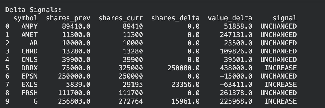
This table transforms raw holdings into directional signals—such as entry, exit, and position scaling—which can be interpreted as changes in institutional conviction across reporting periods.
This step computes the change in holdings between the two filings by calculating the difference in shares and value for each position. These deltas quantify how much a position has increased or decreased across reporting periods.
A classification function is then applied to each row to assign a signal based on how the position has changed. The logic distinguishes between new positions, exits, increases, decreases, and unchanged holdings using the presence and movement of shares.
The final output combines both magnitude (shares and value change) and direction (signal), creating a structured view of portfolio evolution.
Interpretation
The delta signals provide a clear view of how the institution adjusted its portfolio between the two filings. Most positions, such as AMPY, ANET, and CHRD, remain unchanged in terms of share count, indicating stable exposure. When stable share counts are combined with changes in value, the movement is typically driven by market price fluctuations rather than active portfolio reallocation, suggesting passive exposure rather than a shift in institutional conviction.
In contrast, DRRX stands out as a significant increase, with shares rising sharply from 75,000 to 325,000. This indicates a strong increase in conviction and a deliberate capital allocation shift. EXLS and G also show meaningful increases, reinforcing the pattern of selective portfolio expansion.
On the other hand, EPSN shows no change in shares but a decline in value, suggesting that the position faced price pressure during the period. This highlights an important distinction: not all value changes are driven by portfolio decisions.
Overall, the dataset reveals a portfolio that is largely stable with targeted increases in specific positions. This combination of stability and selective reallocation is typical of institutional portfolio management, where broad exposure is maintained while conviction is adjusted at the margin.
Step 5: Build the Final Filing Delta Monitor Table
At this stage, we refine the dataset into a format that is easier to interpret. The goal is to highlight the most meaningful changes by focusing on active signals and sorting positions based on the magnitude of capital movement.
This step improves readability and makes the output more aligned with how analysts review portfolio changes.
|
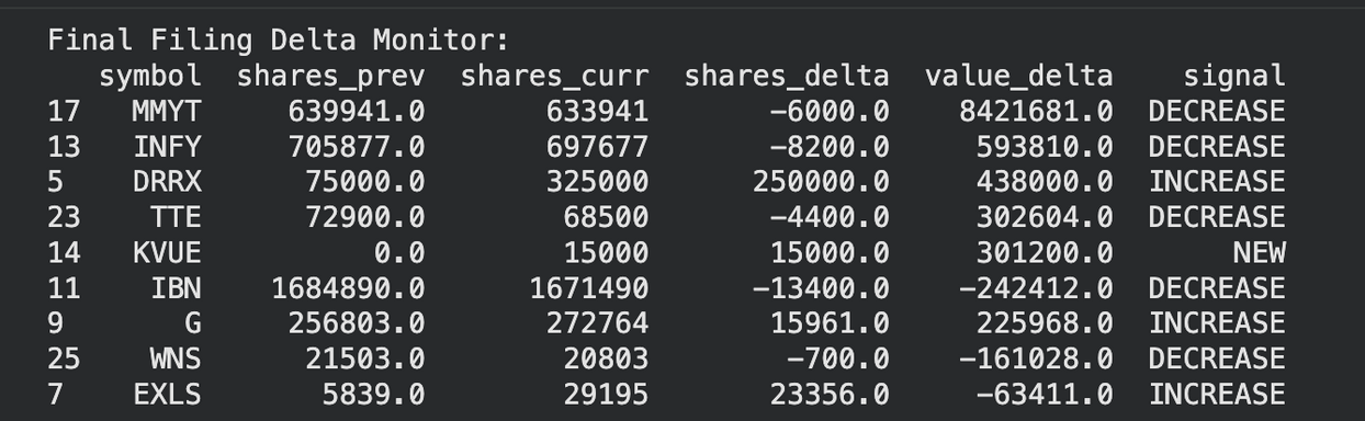
# Filter out unchanged positions df_final = df_merged[df_merged['signal'] != "UNCHANGED"].copy() # Sort by absolute value change (largest moves first) df_final['abs_value_delta'] = df_final['value_delta'].abs() df_final = df_final.sort_values(by='abs_value_delta', ascending=False) # Select final columns df_final = df_final[ ['symbol', 'shares_prev', 'shares_curr', 'shares_delta', 'value_delta', 'signal'] ] print("Final Filing Delta Monitor:") print(df_final.head(10)) |
This final table prioritizes the most meaningful capital movements, making it easier to identify where institutional behavior has materially shifted across positions.
This step refines the merged dataset into an analyst-friendly view by focusing only on positions with meaningful changes. Positions classified as "UNCHANGED" are removed to highlight active portfolio movements.
The dataset is then sorted by the absolute change in value, ensuring that the most significant capital shifts appear at the top. This prioritization helps identify where the institution made its most impactful allocation decisions.
The final table includes key fields such as previous and current shares, the change in shares, the change in value, and the corresponding signal, making it easier to interpret portfolio adjustments.
Interpretation
The final Filing Delta Monitor clearly highlights the most significant portfolio changes between the two filings. MMYT appears as the largest decrease by value, indicating a substantial reduction in exposure despite a relatively small change in share count. This suggests that the position may have experienced strong price appreciation earlier, followed by trimming. Similarly, INFY and IBN show consistent reductions, pointing toward a broader decrease in exposure to certain holdings. In contrast, DRRX stands out as a strong increase, with a sharp rise in both shares and value, indicating a clear increase in conviction. At this stage, an analyst would typically investigate whether these shifts reflect profit-taking, sector rotation, or broader macro-driven allocation changes.
New additions such as KVUE highlight fresh capital deployment, while positions like G and EXLS reflect incremental increases in existing holdings. On the other hand, reductions in WNS suggest selective trimming within the portfolio.
Overall, the portfolio shows a mix of rebalancing and targeted allocation shifts. Large decreases combined with selective increases indicate that the institution is actively redistributing capital rather than making broad structural changes.
Reading Filing Changes
The Filing Delta Monitor converts raw position changes into structured signals, but the real value lies in how these signals are interpreted. Each classification reflects a different type of portfolio behavior and helps analysts understand how institutional conviction evolves over time. In practice, this allows analysts to systematically screen for conviction shifts across filings instead of manually reviewing each report, making the process more scalable and efficient.
In practice, analysts do not treat all changes equally. The combination of signal type and magnitude determines whether a change is meaningful or simply part of routine portfolio maintenance.
Understanding Signal Types
A NEW signal indicates that a position has been introduced in the latest filing. This often reflects fresh conviction or entry into a new theme or sector. Larger value allocations in new positions typically carry stronger significance.
An INCREASE signal shows that an existing position has been expanded. This is generally interpreted as growing confidence, especially when the increase is accompanied by a substantial rise in capital allocation.
A DECREASE signal suggests that the position has been reduced. This may indicate profit booking, risk management, or a shift in portfolio priorities. The magnitude of reduction helps determine whether it is a minor adjustment or a strategic exit in progress.
An EXIT signal represents a complete removal of a position. This is usually considered a strong signal, as it reflects a full withdrawal of capital from that security.
Role of Magnitude in Interpretation
Signals become more meaningful when evaluated alongside the size of the change. A small reduction in shares may not carry much significance, while a large value decrease can indicate a meaningful shift in exposure.
In the case study above, positions like DRRX stand out not just because they are classified as increases, but because of the scale of the change. Similarly, large decreases in positions such as MMYT highlight significant capital reallocation decisions.
This distinction between direction and magnitude is critical for avoiding misleading conclusions.
Separating Market Movement from Portfolio Decisions
It is important to note that not all value changes are driven by active decisions. When share counts remain unchanged but value fluctuates, the change is typically driven by price movement rather than portfolio reallocation.
For example, positions with unchanged shares but increasing value reflect market performance rather than increased conviction. Analysts should focus more on share-based changes when identifying true allocation shifts.
Using the Signal in Practice
The Filing Delta Monitor provides a structured way to track institutional behavior across reporting periods. Analysts can use this signal to:
- identify emerging positions of interest
- track increasing or decreasing conviction
- monitor sector-level allocation trends
- generate ideas for further research
By focusing on changes rather than static holdings, the analysis shifts from descriptive reporting to actionable insight. These signals can be further strengthened by combining them with other datasets such as earnings revisions, price performance, or fundamental metrics, enabling a more comprehensive view of institutional behavior using Financial Modeling Prep's broader data coverage.
Where This Approach Can Mislead
While the Filing Delta Monitor provides a structured view of portfolio changes, it is important to recognize its limitations. The signals reflect what changed, but not necessarily why the change occurred.
One key limitation is the quarterly nature of 13F filings. These filings are reported with a delay, and do not capture intra-quarter trades. A position classified as “NEW” may have been initiated and partially exited within the same quarter, which is not visible in the data.
Another challenge is that value changes can be driven by market movement rather than portfolio decisions. Even when share counts remain constant, fluctuations in price can create the appearance of increased or reduced exposure. Without isolating share-based changes, this can lead to incorrect conclusions.
The approach also does not account for portfolio context. A decrease in one position does not necessarily indicate declining conviction if capital is being reallocated to another opportunity within the same sector or strategy. Similarly, smaller funds may show more volatile changes that do not reflect long-term intent.
Finally, 13F filings include only long equity positions. They do not capture short positions, derivatives, or hedging strategies, which means the overall portfolio exposure may differ significantly from what is observed.
Because of these limitations, the Filing Delta Monitor should be used as a directional signal, not a definitive indicator of investment intent.
Turning Filings Into Actionable Signals
The Filing Delta Monitor transforms static 13F filings into a structured view of portfolio change. By comparing two reporting periods, it highlights where institutions are adding exposure, reducing positions, or reallocating capital.
The framework is most useful for identifying conviction shifts and emerging positions, especially when combined with the magnitude of change. Large increases, new entries, and significant exits often provide stronger signals than stable holdings.
At the same time, the signal should be interpreted with context. Filing delays, market-driven value changes, and incomplete portfolio visibility can influence the output. As a result, the Filing Delta Monitor is best used as a starting point for deeper analysis, rather than a standalone decision tool.
To extend this analysis across multiple institutions or longer time horizons, access to consistent and structured filing data is essential. Financial Modeling Prep provides this through its APIs, which can be explored further on their pricing page for broader usage and scaling this framework. In practice, this framework can be scaled across funds to build systematic screens that identify emerging conviction shifts and capital rotation patterns in institutional portfolios.
FAQs
1. What is a Filing Delta Monitor?
A Filing Delta Monitor is a framework that compares two institutional filings to identify how portfolio positions have changed over time. It highlights new positions, exits, and changes in exposure.
2. Why are 13F filings useful for this analysis?
13F filings provide structured, position-level data for institutional investors. This makes them ideal for tracking changes in holdings across reporting periods in a consistent and comparable format.
3. What does a “NEW” or “EXIT” signal indicate?
A “NEW” signal means the institution has initiated a position in the latest filing, while an “EXIT” signal indicates that the position has been completely removed from the portfolio.
4. How should increases and decreases in positions be interpreted?
An increase typically reflects growing conviction, while a decrease may indicate profit booking, risk reduction, or portfolio rebalancing. The magnitude of change helps determine its significance.
5. Can value changes alone indicate portfolio decisions?
Not always. Changes in value can be driven by market price movements even if the number of shares remains the same. Share-based changes provide a clearer signal of actual portfolio activity.
6. What are the limitations of using 13F data?
13F filings are reported quarterly and with a delay. They also include only long equity positions and do not capture short positions, derivatives, or intra-quarter trades.
7. How can this framework be extended further?
The Filing Delta Monitor can be scaled across multiple institutions, time periods, or sectors. It can also be combined with other financial data to build more advanced investment signals.

Financial APIs, Claude MCP, and AI-driven research workflows
Pranjal Saxena writes technical content focused on financial data APIs, Claude MCP workflows, AI-driven research systems, and Python-based market analysis. For FMP, his work centers on turning structured financial data into practical, workflow-driven content for developers, analysts, and fintech teams. He combines experience in data science, NLP, generative AI, and financial API workflows to show how APIs, automation, and AI-assisted systems can support modern financial research and analysis.
Related




Financial data for every need
Real-time quotes and 30+ years of historical data, including prices, fundamentals, and insider transactions — all accessible via API.
Create Free Account