How to Measure Analyst Estimate Dispersion and Forecast Uncertainty

Two equities can have the exact same consensus forward estimate but vastly different levels of agreement among the analysts covering them. An expected EPS of 3.50 derived from twenty analysts modeling within a tight ten-cent band implies stability, while that same 3.50 average drawn from forecasts ranging from 1.00 to 6.00 signals a fragmented narrative.
Consensus averages routinely simplify complex financial models into a single digestible data point. This mathematical aggregation inherently hides disagreement across research desks regarding macroeconomic exposure, product cycle viability, or margin resilience. Relying purely on consensus expectations without checking the variance leaves valuation models exposed to hidden structural risks.
Dispersion measures exactly how much analysts disagree, capturing the spread or variance around that consensus mean. Tracking this variability provides a critical but often overlooked signal of fundamental risk that standard terminal screens miss.
This page explains how to retrieve or calculate estimate dispersion programmatically, how to interpret it accurately, and how it fits into real-world institutional analysis and risk management pipelines. In institutional workflows, dispersion is not just a descriptive statistic. It is a dynamic signal derived from structured analyst datasets and monitored over time.
How Can I Fetch Estimates Dispersion and Standard Deviation Metrics?
Estimates dispersion and standard deviation metrics are sometimes available through financial data APIs, but are often not provided directly and must be calculated from individual analyst estimates. Structured APIs provide the underlying estimate distributions that allow internal systems to compute and track dispersion programmatically.
Dispersion mathematically represents the width of the expectation distribution. It captures two primary concepts:
- The absolute range of analyst estimates from the highest projection to the lowest
- The statistical variability or standard deviation around the consensus mean
Developers must clarify the difference between APIs that deliver precomputed standard deviation metrics and those that provide the raw individual estimates required to build internal variance models. Financial Modeling Prep serves as a structured API provider that enables this workflow by delivering the raw consensus boundaries needed to power these internal calculations.
If dispersion is not available, it can be calculated using the distribution of analyst estimates for a given metric such as EPS or revenue. Querying endpoints like the Price Target Consensus API provides the high, low, and median values needed to establish this baseline spread across the street.

How to Calculate Dispersion from Analyst Estimates
Calculating dispersion requires extracting the outer boundaries of street expectations. Analysts typically utilize specific statistical methods to quantify this disagreement for internal modeling.
The basic methods for calculating this variance include:
- Standard deviation, which measures the average distance of each individual estimate from the mean
- Absolute range, which simply subtracts the lowest street estimate from the highest
Standard deviation provides a much more stable measure than a simple absolute range because it accounts for the clustering of estimates and prevents a single extreme outlier from skewing the entire risk profile.
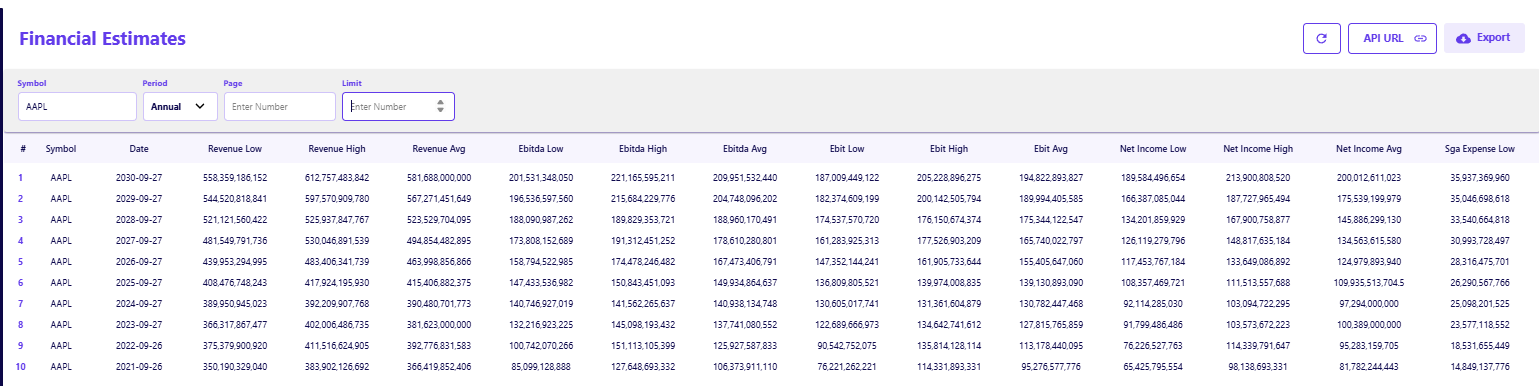
Consider a case where a company carries a consensus EPS of 2.50. If the underlying estimates range from 2.10 to 2.90, this wide 80-cent band implies substantial institutional disagreement regarding margins or growth sustainability. Extracting these exact boundaries programmatically via the Financial Estimates API allows quants to identify when a significant portion of the street will be wrong regardless of the reported number. Rather than manually checking these ranges, quantitative teams build automated data pipelines that continuously ingest these boundaries and update internal risk scores without human intervention.
Why Dispersion Matters More Than the Consensus Average
The consensus number alone does not reflect the uncertainty embedded in a forward financial model. It provides a static target but strips away the context of institutional conviction.
Evaluating the distribution reveals the true narrative:
- Tight clustering around the mean indicates strong agreement on macroeconomic exposure and execution
- Wide dispersion reveals divergent assumptions about cost structures, terminal growth rates, or regulatory headwinds
High dispersion often signals elevated uncertainty, fundamental disagreement, and a significantly higher potential for an earnings surprise. When models vary wildly, the pricing efficiency of the underlying equity drops.
In practical application, high dispersion translates directly to less confidence in the forecast, demanding a higher risk premium. Conversely, low dispersion implies stronger agreement and a higher probability that the equity will trade cleanly on fundamentals.
Tracking how dispersion changes over time is just as critical as measuring its absolute width. A tightening dispersion indicates that analysts are reaching a stronger consensus, reducing the likelihood of a surprise. Conversely, a widening dispersion signals rising uncertainty and a fracturing of the corporate narrative, warning systems that fundamental risk is increasing.
How Analysts Use Dispersion in Real Decision-Making
Quantitative and discretionary teams integrate dispersion metrics directly into their daily workflows to manage exposure. Dispersion is systematically used in several critical applications. These signals are typically integrated into systematic models that continuously ingest analyst data and update risk metrics in real time.
Dispersion is systematically used in several critical applications:
- Earnings risk assessment models to predict implied volatility ahead of reporting dates
- Position sizing algorithms that scale down notional exposure when standard deviation expands
- Alpha screening systems hunting for mispriced equities and notable price target gaps exhibiting high uncertainty
Elevated dispersion can signal potential volatility or a fundamental disagreement in the corporate narrative that terminal screens miss.
Consider a realistic scenario where a software company experiences steadily rising consensus estimates, but the dispersion of those estimates is simultaneously increasing. This dynamic is highly complex because it indicates that while the average outlook is improving, the street is becoming violently split on the actual magnitude of the upside. Identifying this divergence is crucial when building systematic momentum signals to avoid false breakouts.
The Limitations of Consensus-Based Analysis
Relying exclusively on the mean estimate treats the consensus as an objective truth rather than a mathematical compromise. This binary approach ignores the reality that institutional research desks rarely agree on the granular inputs of a discounted cash flow model.
Institutional disagreement is often far more informative than the average itself. Tracking how the spread widens or narrows provides real-time context that the isolated consensus number simply cannot communicate.
Consensus is a summary, but dispersion reveals the underlying uncertainty. Recognizing this distinction allows risk managers to separate high-conviction forecasts from fragile mathematical averages when they compare forward KPIs across sector peers. Evaluating how these ranges shift over time using the Price Target Summary API helps developers map this uncertainty across longer market cycles. By returning aggregated historical target counts and average prices over distinct trailing periods, this API enables analytical models to track precisely when and how street conviction began to drift.

How to Use Dispersion Without Overcomplicating Your Analysis
Tracking estimate variance is highly situational and should be applied where it yields the highest signal-to-noise ratio.
Dispersion is most useful during:
- Volatile earnings periods where guidance shifts are expected
- Analysis of uncertain industries like biotechnology or emerging technology
- Major macroeconomic transitions that disrupt historical cash flow models
It may be less critical for mature, highly regulated utility companies where cash flows are contracted and analyst models exhibit minimal variance. Applying complex standard deviation calculations across a stable, low-beta portfolio often introduces unnecessary computational overhead.
Quantitative teams should encourage using variance as a complementary risk signal to dynamically adjust discount rates within existing research pipelines and actively monitor target price changes to protect portfolio downside. Dispersion should be used to understand confidence, not to replace the consensus itself. In modern research systems, dispersion is continuously tracked alongside consensus to monitor how confidence evolves in real time.
Frequently Asked Questions
What causes high estimate dispersion?
High dispersion typically stems from fundamental uncertainty regarding a company's future. This occurs during major macroeconomic shifts, management transitions, unproven product launches, or when a company issues ambiguous forward guidance that forces analysts to make disparate assumptions.
How does dispersion affect implied volatility?
Equities with high analyst dispersion generally command higher implied volatility in the options market. Because the street cannot agree on a fundamental baseline, market makers price in a wider expected move around binary events like earnings announcements to account for the heightened risk of a surprise.
Should I avoid stocks with high estimate dispersion?
Not necessarily. While high dispersion indicates higher risk and lower confidence in the consensus, it also creates the environment for significant mispricing. Quantitative funds often screen for high dispersion because correctly anticipating the resolution of that disagreement can generate substantial returns.
Why is standard deviation preferred over absolute range?
Absolute range only measures the distance between the single highest and single lowest estimate, making it highly sensitive to one rogue analyst model. Standard deviation measures how all estimates cluster around the mean, providing a much more accurate representation of overall street consensus and systemic variance.
Do all financial APIs provide precomputed dispersion?
No. Many financial APIs focus on delivering the consensus mean or the raw individual analyst estimates. To acquire dispersion metrics, data engineering teams often ingest the high, low, and median boundaries from the API payload and calculate the standard deviation internally.

Risk analysis and financial modeling for data-driven market workflows
Parth Sanghvi is a Senior Risk Consultant with experience in financial modeling, valuation, and risk analysis. For FMP, he focuses on translating complex market data and risk models into clear, accessible analysis for developers and investors. His work centers on helping readers understand how institutional-grade financial data applies to real-world workflows and decision-making.
Related




Financial data for every need
Real-time quotes and 30+ years of historical data, including prices, fundamentals, and insider transactions — all accessible via API.
Create Free Account